HicAggR - In depth tutorial • HicAggR

Introduction

HicAggR package provides a set of tools for the analysis of genomic 3D conformation data (HiC). It is designed around Aggregation Peak Analysis (APA), with the intent to provide easy-to-use sets of functions that would allow users to integrate 1D-genomics data with 3D-genomics data. This package does not perform TAD calling, loop calling, or compartment analysis. There are other packages available for these analyses (eg: TopDom (from CRAN), HiTC (bioconductor), HiCDOC (bioconductor)…). The package offers however tools to perform downstream analyses on called loops,or make use of called TADs to explore interactions within loops or explore intra/inter-TAD interactions. To this end, pixels of interest surrounding called loops or genomic features are extracted from whole HiC matrices (as submatrices), abiding to TAD and/or compartmental constraints in order to give user an insight into the interaction patterns of features of interest or called loops.

Typical workflow:

The straight-forward workflow with this package would be:

to import genomic coordinates of features of interest (such as, enhancers, CTCF binding sites, genes) as GRanges
apply distance constraints or 3D structural constraints (like TADs) to form all potential couples between features of interest under the applied contraints. (Enhancer-promoter, CTCF-CTCF etc.)
import 3D-genomics data (.hic, bedpe, h5, cool/mcool formats).
perform matrix balancing and distance normalization if necessary.
extract submatrices of the pre-formed potential couples from the 3D-genomics Data.
perform corrections per-submatrix
1. orientation correction: i.e. set one feature of interest per axe which is to capture a uniform pattern for interactions that are towards upstream or downstream.
2. ranking pixels per submatrix to highligt the most significant interaction signals per submatrix.
summarize visually the genome-wide interactions between features of interest graphically through APA
and/or get individual values of selected zones from each submatrix for comparison between conditions

We also propose (since version 0.99.3) a function to find couples that demonstrate a non-random (or non-background) like interaction signals. The function performs z.test to compare target couples to less-plausible or background couples to identify target couples with significantly higher interaction values than the background signal (compareToBackground).

Quickstart and tutorials:

Please visit dedicated github pages and the github repository.

Aim:

The principal objective is to simplify the extraction of interaction signals from HiC data, by making submatrices easy to access and treat if necessary. As such the contact matrices are imported as a list of ContactMatrix objects per combination of chromosomes(eg: “chr1_chr1” or “chr1_chr2”). This allows the user to access the data easily for dowstream analyses.

Requirements

Installation

The bioconductor release version:

if (!requireNamespace("BiocManager", quietly = TRUE))
    install.packages("BiocManager")

BiocManager::install("HicAggR")

The developmental version:

remotes::install_github("CuvierLab/HicAggR")

Load library

library("HicAggR")

Test dataset

Description

Data were obtained from Drosophila melanogaster S2 cells. 1. HiC test dataset Directly downloaded from the 4DN platform. * Control Condition
* Heat Shock Condition
2. Genomic coordinates:
* ChIPseq peaks of Beaf-32 protein in wild type cells (GSM1278639). * Reference annotation data for TSS from the UCSC database.
* Topologically associating domains (TAD) annotations were defined as described (F. Ramirez, 2018).

1. Genomic 3D structure

For a test, please download HiC data in .hic format (Juicer) and .mcool format (HiCExplorer). Examples for each format are provided below.

Temp directory preparation

withr::local_options(list(timeout = 3600))
# temp.dir <- file.path(tempdir(), "HIC_DATA")
cache.dir <- paste0(tools::R_user_dir("", which="cache"),".HicAggR_HIC_DATA")
bfc <- BiocFileCache::BiocFileCache(cache.dir,ask = FALSE)
# dir.create(temp.dir)

Control condition (.hic File)

if(length(BiocFileCache::bfcinfo(bfc)$rname)==0 ||
    !"Control_HIC.hic"%in%BiocFileCache::bfcinfo(bfc)$rname){
    Hic.url <- paste0("https://4dn-open-data-public.s3.amazonaws.com/",
        "fourfront-webprod/wfoutput/7386f953-8da9-47b0-acb2-931cba810544/",
        "4DNFIOTPSS3L.hic")
    if(.Platform$OS.type == "windows"){
        HicOutput.pth <- BiocFileCache::bfcadd(
            x = bfc,rname = "Control_HIC.hic",
            fpath = Hic.url,
            download = TRUE,
            config = list(method="auto",mode="wb"))
    }else{
        HicOutput.pth <- BiocFileCache::bfcadd(
            x = bfc, rname = "Control_HIC.hic",
            fpath = Hic.url,
            download = TRUE,
            config = list(method="auto"))
    }
}else{
    HicOutput.pth <- BiocFileCache::bfcpath(bfc)[
        which(BiocFileCache::bfcinfo(bfc)$rname=="Control_HIC.hic")]
}

Heat shock condition (.mcool File)

if(length(BiocFileCache::bfcinfo(bfc)$rname)==0 ||
    !"HeatShock_HIC.mcool"%in%BiocFileCache::bfcinfo(bfc)$rname){
    Mcool.url <- paste0("https://4dn-open-data-public.s3.amazonaws.com/",
        "fourfront-webprod/wfoutput/4f1479a2-4226-4163-ba99-837f2c8f4ac0/",
        "4DNFI8DRD739.mcool")
    if(.Platform$OS.type == "windows"){
        McoolOutput.pth <- BiocFileCache::bfcadd(
            x = bfc, rname = "HeatShock_HIC.mcool",
            fpath = Mcool.url,
            download = TRUE,
            config = list(method="auto",mode="wb"))
    }else{
        McoolOutput.pth <- BiocFileCache::bfcadd(
            x = bfc, rname = "HeatShock_HIC.mcool",
            fpath = Mcool.url,
            download = TRUE,
            config = list(method="auto"))
    }
}else{
    McoolOutput.pth <- as.character(BiocFileCache::bfcpath(bfc)[
        which(BiocFileCache::bfcinfo(bfc)$rname == "HeatShock_HIC.mcool")])
}

2 Genomic location and annotation data

These kind of data can be imported in R with rtracklayer package.

ChIPseq peaks of Beaf-32 protein

data("Beaf32_Peaks.gnr")

View

seq	start	end	strand	name	score
2L	35594	35725	*	Beaf32_2	76
2L	47296	47470	*	Beaf32_3	44
2L	65770	65971	*	Beaf32_5	520

TSS annontation

data("TSS_Peaks.gnr")

View

seq	start	end	strand	name	class
2L	71757	71757	+	FBgn0031213	active
2L	76348	76348	+	FBgn0031214	inactive
2L	106903	106903	+	FBgn0005278	active

TADs annotation

data("TADs_Domains.gnr")

View

seq	start	end	strand	name	score	class
2L	73104	94543	*	Tad_1	3	active
2L	94544	102930	*	Tad_2	8	active
2L	102931	121473	*	Tad_3	8	active

Additional genome informations

Required genomic informations used by the functions during the entire pipeline are a data.frame containing chromosomes names and sized and the binSize, corresponding to the HiC matrices at the same resolution.

seqlengths.num <- c('2L'=23513712, '2R'=25286936)
chromSizes  <- data.frame(
    seqnames   = names(seqlengths.num ), 
    seqlengths = seqlengths.num
    )
binSize <- 5000

Import HiC

The package supports the import and normalization of HiC data.

NOTE: Since version 0.99.2, the package supports import of balanced HiC matrices in .hic, .cool/.mcool formats. It also supports the import of ‘o/e’ matrices in .hic format.

Import

HicAggR can import HiC data stored in the main formats: .hic, .cool, .mcool, .h5 (since version 0.99.2). The pacakage imports by default the raw counts. Therefore, it is necessary to perform the balancing and observed/expected correction steps.

HiC_Ctrl.cmx_lst <- ImportHiC(
        file    = HicOutput.pth,
        hicResolution     = 5000,
        chrom_1 = c("2L", "2L", "2R"),
        chrom_2 = c("2L", "2R", "2R")
)

HiC_HS.cmx_lst <- ImportHiC(
        file    = McoolOutput.pth,
        hicResolution     = 5000,
        chrom_1 = c("2L", "2L", "2R"),
        chrom_2 = c("2L", "2R", "2R")
)

Balancing

The balancing is done such that every bin of the matrix has approximately the same number of contacts within the contactMatrix.

HiC_Ctrl.cmx_lst <- BalanceHiC(HiC_Ctrl.cmx_lst)
HiC_HS.cmx_lst <- BalanceHiC(HiC_HS.cmx_lst)

Tips

In the interactionType parameter it is required to define “cis” or “trans”. Then the function will return only ContactMatrices in the corresponding category (“cis” or “trans”). All other categories will be removed from the result.
In the interactionType parameter if you type c(“cis”,“trans”) the function will normalize separetly “cis” or “trans”. If you type “all” the function will normalize “cis” and “trans” matrices together.

Observed/Expected Correction

To correct effects due to genomic distance the matrix is corrected by the expected values for each genomic distance. The expected values are by default calculated as the average values of contacts per chromosome and per distance.

NOTE: Since version 0.99.3, 2 more options to calculate expected values have been implemented. We designated the methods as the “lieberman” and the “mean_total”. These methods were implemented based on the options proposed by HiCExplorer’s hicTransform program. The “lieberman” method computes per distance (d) expected values by dividing the sum of all contacts by the difference of chromosome length and distance(d).

The “mean_total” is simply the average of all contact values including 0 values, which are ignored in the default method (“mean_non_zero”)

HiC_Ctrl.cmx_lst <- OverExpectedHiC(HiC_Ctrl.cmx_lst)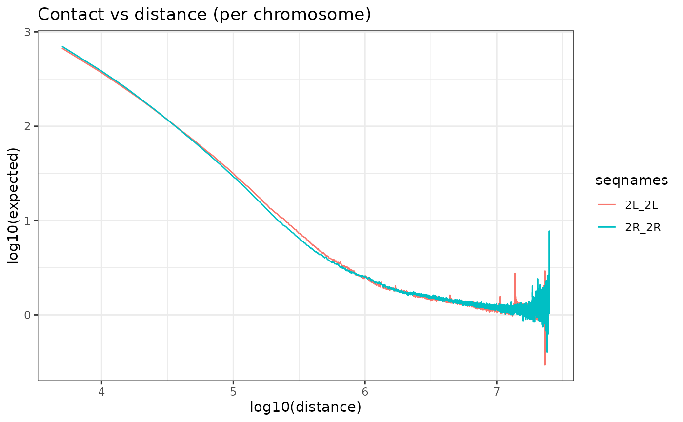

HiC_HS.cmx_lst <- OverExpectedHiC(HiC_HS.cmx_lst)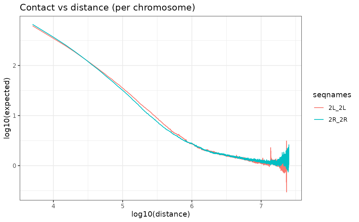

Tips

After runing OverExpectedHiC function, expected counts can be plotted as a function of genomic distances with tibble by taking the expected attributes.

HiC data format: ContactMatrix list structure

Each element of the list corresponds to a ContactMatrix object (dgCMatrix object, sparse matrix format) storing contact frequencies for one chromosome (cis-interactions, ex: “2L_2L”) or between two chromosomes (trans-interactions, ex: “2L_2R”). HiC data format is based on InteractionSet and Matrix packages.

str(HiC_Ctrl.cmx_lst,max.level = 4)
#> List of 3
#>  $ 2L_2L:Formal class 'ContactMatrix' [package "InteractionSet"] with 5 slots
#>   .. ..@ matrix  :Formal class 'dgCMatrix' [package "Matrix"] with 6 slots
#>   .. ..@ anchor1 : int [1:4703] 1 2 3 4 5 6 7 8 9 10 ...
#>   .. ..@ anchor2 : int [1:4703] 1 2 3 4 5 6 7 8 9 10 ...
#>   .. ..@ regions :Formal class 'GRanges' [package "GenomicRanges"] with 7 slots
#>   .. ..@ metadata:List of 10
#>   .. .. ..$ name         : chr "2L_2L"
#>   .. .. ..$ type         : chr "cis"
#>   .. .. ..$ kind         : chr "U"
#>   .. .. ..$ symmetric    : logi TRUE
#>   .. .. ..$ resolution   : num 5000
#>   .. .. ..$ expected     : num [1:2410023] 719 673 719 370 673 ...
#>   .. .. ..$ removedCounts:Formal class 'dgCMatrix' [package "Matrix"] with 6 slots
#>   .. .. ..$ observed     : num [1:2410023] 1329 1721 1852 1076 2191 ...
#>   .. .. ..$ normalizer   : num [1:2410023] 1.399 1.115 0.888 1.139 0.908 ...
#>   .. .. ..$ mtx          : chr "norm"
#>  $ 2L_2R:Formal class 'ContactMatrix' [package "InteractionSet"] with 5 slots
#>   .. ..@ matrix  :Formal class 'dgCMatrix' [package "Matrix"] with 6 slots
#>   .. ..@ anchor1 : int [1:4703] 1 2 3 4 5 6 7 8 9 10 ...
#>   .. ..@ anchor2 : int [1:5058] 4704 4705 4706 4707 4708 4709 4710 4711 4712 4713 ...
#>   .. ..@ regions :Formal class 'GRanges' [package "GenomicRanges"] with 7 slots
#>   .. ..@ metadata:List of 9
#>   .. .. ..$ name         : chr "2L_2R"
#>   .. .. ..$ type         : chr "trans"
#>   .. .. ..$ kind         : chr NA
#>   .. .. ..$ symmetric    : logi FALSE
#>   .. .. ..$ resolution   : num 5000
#>   .. .. ..$ removedCounts:Formal class 'dgCMatrix' [package "Matrix"] with 6 slots
#>   .. .. ..$ observed     : num [1:1292193] 1 1 1 1 1 1 1 1 1 1 ...
#>   .. .. ..$ normalizer   : num [1:1292193] 2.73 2.82 2.78 2.48 4.4 ...
#>   .. .. ..$ expected     : num 0.0596
#>  $ 2R_2R:Formal class 'ContactMatrix' [package "InteractionSet"] with 5 slots
#>   .. ..@ matrix  :Formal class 'dgCMatrix' [package "Matrix"] with 6 slots
#>   .. ..@ anchor1 : int [1:5058] 1 2 3 4 5 6 7 8 9 10 ...
#>   .. ..@ anchor2 : int [1:5058] 1 2 3 4 5 6 7 8 9 10 ...
#>   .. ..@ regions :Formal class 'GRanges' [package "GenomicRanges"] with 7 slots
#>   .. ..@ metadata:List of 10
#>   .. .. ..$ name         : chr "2R_2R"
#>   .. .. ..$ type         : chr "cis"
#>   .. .. ..$ kind         : chr "U"
#>   .. .. ..$ symmetric    : logi TRUE
#>   .. .. ..$ resolution   : num 5000
#>   .. .. ..$ expected     : num [1:2769177] 746 703 746 152 192 ...
#>   .. .. ..$ removedCounts:Formal class 'dgCMatrix' [package "Matrix"] with 6 slots
#>   .. .. ..$ observed     : num [1:2769177] 374 368 614 95 131 420 18 17 26 332 ...
#>   .. .. ..$ normalizer   : num [1:2769177] 2.62 2.19 1.84 2.94 2.46 ...
#>   .. .. ..$ mtx          : chr "norm"
#>  - attr(*, "resolution")= num 5000
#>  - attr(*, "chromSize")= tibble [2 × 3] (S3: tbl_df/tbl/data.frame)
#>   ..$ name     : chr [1:2] "2L" "2R"
#>   ..$ length   : num [1:2] 23513712 25286936
#>   ..$ dimension: num [1:2] 4703 5058
#>  - attr(*, "matricesKind")= tibble [3 × 4] (S3: tbl_df/tbl/data.frame)
#>   ..$ name     : chr [1:3] "2L_2L" "2L_2R" "2R_2R"
#>   ..$ type     : chr [1:3] "cis" "trans" "cis"
#>   ..$ kind     : chr [1:3] "U" NA "U"
#>   ..$ symmetric: logi [1:3] TRUE FALSE TRUE
#>  - attr(*, "mtx")= chr "o/e"
#>  - attr(*, "expected")= tibble [4,961 × 2] (S3: tbl_df/tbl/data.frame)
#>   ..$ distance: num [1:4961] 1 5001 10001 15001 20001 ...
#>   ..$ expected: num [1:4961] 733 689 377 257 191 ...

#>

The list has the attributes described below. These attributes are accessible via:

attributes(HiC_Ctrl.cmx_lst)
#> $names
#> [1] "2L_2L" "2L_2R" "2R_2R"
#> 
#> $resolution
#> [1] 5000
#> 
#> $chromSize
#> # A tibble: 2 × 3
#>   name    length dimension
#>   <chr>    <dbl>     <dbl>
#> 1 2L    23513712      4703
#> 2 2R    25286936      5058
#> 
#> $matricesKind
#> # A tibble: 3 × 4
#>   name  type  kind  symmetric
#>   <chr> <chr> <chr> <lgl>    
#> 1 2L_2L cis   U     TRUE     
#> 2 2L_2R trans NA    FALSE    
#> 3 2R_2R cis   U     TRUE     
#> 
#> $mtx
#> [1] "o/e"
#> 
#> $expected
#> # A tibble: 4,961 × 2
#>   distance expected
#>      <dbl>    <dbl>
#> 1        1     733.
#> 2     5001     689.
#> 3    10001     377.
#> 4    15001     257.
#> # ℹ 4,957 more rows

#>

names : the names of list elements (ContactMatrix).
resolution : the resolution of the HiC map.
chromSize : the size of the chromosomes in the tibble format.
- seqnames : the sequence name (chromosome name).
- seqlengths : the sequence length in base pairs.
- dimension : the sequence length in number of bins.
matricesKind : the kind of matrix that composes the list in the tibble format.
- name : the matrix name. - type : interactionType. “Cis” for interactions on the same chromosome and “Trans” for interactions on different chromosomes. - kind : the matrix kind. U for upper triangle matrices, L for lower triangle matrices, NA for rectangular or square matrices. - symmetric : a boolean that indicates whether the matrix is symmetric (lower triangle identical to upper triangle).
mtx : the kind of values in matrix. For exemple observed counts, normalized counts, observed/expected, etc.
expected : This attribute is related to the OverExpectedHiC function. It gives a tibble with the expected counts as a function of genomic distance.

Each contactmatrix in the list have metadata. These are accessible via:

str(S4Vectors::metadata(HiC_Ctrl.cmx_lst[["2L_2L"]]))
#> List of 10
#>  $ name         : chr "2L_2L"
#>  $ type         : chr "cis"
#>  $ kind         : chr "U"
#>  $ symmetric    : logi TRUE
#>  $ resolution   : num 5000
#>  $ expected     : num [1:2410023] 719 673 719 370 673 ...
#>  $ removedCounts:Formal class 'dgCMatrix' [package "Matrix"] with 6 slots
#>   .. ..@ i       : int [1:266585] 2 10 18 19 20 28 32 37 38 40 ...
#>   .. ..@ p       : int [1:4704] 0 0 0 0 0 0 0 0 0 0 ...
#>   .. ..@ Dim     : int [1:2] 4703 4703
#>   .. ..@ Dimnames:List of 2
#>   .. .. ..$ : NULL
#>   .. .. ..$ : NULL
#>   .. ..@ x       : num [1:266585] 1 1 1 2 1 1 1 1 1 2 ...
#>   .. ..@ factors : list()
#>  $ observed     : num [1:2410023] 1329 1721 1852 1076 2191 ...
#>  $ normalizer   : num [1:2410023] 1.399 1.115 0.888 1.139 0.908 ...
#>  $ mtx          : chr "norm"

#>

name : the name of the ContactMatrix.
type : interactionType. “Cis” for interactions on the same chromosome and “Trans” for interactions on different chromosomes (or arms).
kind : the matrix kind. U for upper triangle matrices, L for lower triangle matrices, NA for rectangular or square
symmetric : a boolean that indicates whether the matrix is symmetric (lower triangle identical to upper triangle).
resolution : resolution of the HiC map.
removedCounts : A sparse matrix (dgCMatrix) of the removed counts (counts that are below the threshold on rows or columns as described in BalanceHiC).
observed : observed counts of the sparse matrix.
normalizer : the balancer vector that converts the observed counts into normalized counts. (observed * normalizer = normalized counts).
mtx : the kind of values in matrix. For example observed counts, normalized counts, observed/expected, etc.
expected : This attributes is related to the OverExpectedHiC function. It gives the expected vector that convert the normalized counts into the observed/expected counts (normalized counts / expected = observed/expected).

Indexing

This part of the data corresponds to the positioning data (ChIPseq peaks, genomic features and annotations, genes, etc) on the genome. To integrate such annotations with HiC data in 2D matrices, annotations must be processed as followed.

The first step is the indexing of the features. It allows the features to be splitted and grouped into bins corresponding to the HiC bin size.

Example 1: Anchors from Beaf32 ChIP-seq peaks (bed file)

anchors_Index.gnr <- IndexFeatures(
    gRangeList        = list(Beaf=Beaf32_Peaks.gnr), 
    genomicConstraint        = TADs_Domains.gnr,
    chromSizes         = chromSizes,
    binSize           = binSize,
    metadataColName = "score",
    method            = "max"
    )

View

seqnames	start	end	width	strand	name	bin	constraint	Beaf.score	Beaf.name	Beaf.bln
2L	70001	75000	5000	*	2L:15:Tad_1	2L:15	Tad_1	205	Beaf32_8	TRUE
2L	100001	105000	5000	*	2L:21:Tad_2	2L:21	Tad_2	1830	Beaf32_11	TRUE
2L	110001	115000	5000	*	2L:23:Tad_3	2L:23	Tad_3	1707	Beaf32_14	TRUE

Example 2: Baits from TSS (transcription start sites from UCSC)

baits_Index.gnr <- IndexFeatures(
    gRangeList        = list(Tss=TSS_Peaks.gnr),
    genomicConstraint        = TADs_Domains.gnr,
    chromSizes         = chromSizes,
    binSize           = binSize,
    metadataColName = "score",
    method            = "max"
    )

View

seqnames	start	end	width	strand	name	bin	constraint	Tss.class	Tss.name	Tss.bln
2L	75001	80000	5000	*	2L:16:Tad_1	2L:16	Tad_1	inactive	FBgn0031214	TRUE
2L	105001	110000	5000	*	2L:22:Tad_3	2L:22	Tad_3	active	FBgn0026….	TRUE
2L	115001	120000	5000	*	2L:24:Tad_3	2L:24	Tad_3	active	FBgn0031219	TRUE

Filter indexed features:

By using features names and bin IDs, it is possible to filter a subset of features. Example: Subset TSS that are not in the same bin than a Beaf32 peak.

non_Overlaps.ndx <- match(baits_Index.gnr$bin, 
    anchors_Index.gnr$bin, nomatch=0L)==0L
baits_Index.gnr <- baits_Index.gnr[non_Overlaps.ndx,]

View

seqnames	start	end	width	strand	name	bin	constraint	Tss.class	Tss.name	Tss.bln
2L	75001	80000	5000	*	2L:16:Tad_1	2L:16	Tad_1	inactive	FBgn0031214	TRUE
2L	105001	110000	5000	*	2L:22:Tad_3	2L:22	Tad_3	active	FBgn0026….	TRUE
2L	115001	120000	5000	*	2L:24:Tad_3	2L:24	Tad_3	active	FBgn0031219	TRUE

Tips

It is possible to index multiple features at the same time by submitting a named list of GRanges. Names given in the list of GRanges can then be used to filter indexed features and pairs.
If genomicConstraint is defined, then anchors and baits will be paired when located within the same region only. If contraint.gnr is NULL, entire chromosomes (or arms) are used as constraints.
When multiple ranges are in a same bin (ex: 3 ChIP-seq peaks in the same 10kb bin), associated numeric variables in metadata (metadataColName) can be summarized according to the defined method (method), Example: Max peak score of the bin is kept in metadata column score.

Search Pairs

Pairing

SearchPairs function takes as input one or two indexed features and returns all putative pairs within the same constraint (ex: wihtin the same TAD).
If only one indexed features is defined in indexAnchor, SearchPairs will return symetrical homotypic pairs (A<->A), if indexAnchor and indexBait are defined, it will return asymetrical heterotypic pairs (A<->B).

interactions.gni <- SearchPairs(
        indexAnchor = anchors_Index.gnr,
        indexBait   = baits_Index.gnr
        )

View

Ranges						Metadata
First			Second			Interaction					Anchor					Bait
seq	start	end	seq	start	end	name	constraint	distance	orientation	submatrix.name	name	bin	Beaf.name	Beaf.score	Beaf.bln	name	bin	Tss.name	Tss.class	Tss.bln
2L	70001	75000	2L	75001	80000	2L:15_2L:16	Tad_1	5000	TRUE	2L:15_2L:16	2L:15:Tad_1	2L:15	Beaf32_8	205	TRUE	2L:16:Tad_1	2L:16	FBgn0031214	inactive	TRUE
2L	110001	115000	2L	105001	110000	2L:23_2L:22	Tad_3	5000	FALSE	2L:22_2L:23	2L:23:Tad_3	2L:23	Beaf32_14	1707	TRUE	2L:22:Tad_3	2L:22	FBgn0026….	active	TRUE
2L	120001	125000	2L	105001	110000	2L:25_2L:22	Tad_3	15000	FALSE	2L:22_2L:25	2L:25:Tad_3	2L:25	Beaf32_15	484	TRUE	2L:22:Tad_3	2L:22	FBgn0026….	active	TRUE

Tips

If indexBait is NULL, SearchPairs will return homotypic pairs with indexAnchor.
Minimum and maximum distances between pairs anchors can be set. Note that it is also possible to filter pairs within a specific distance later on.

Extractions

Case 1: Long-range interactions between two distal anchors.

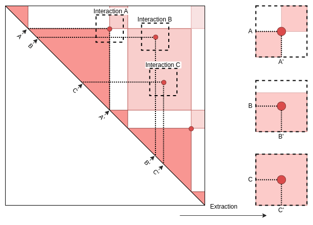
Interactions defined with GInteraction or Pairs of GRanges.

In extracted matrices, the middle of the Y axis corresponds to the center of the first element and interacts with the center of second element in the middle of the X axis.

interactions_PFmatrix.lst <- ExtractSubmatrix(
    genomicFeature         = interactions.gni,
    hicLst        = HiC_Ctrl.cmx_lst,
    referencePoint = "pf",
    matriceDim     = 41
    )

Interactions defined with GRanges.

The middle of the Y axis corresponds to the start of the range and interacts with the middle of the X axis which corresponds to the end of the range.

domains_PFmatrix.lst <- ExtractSubmatrix(
    genomicFeature         = TADs_Domains.gnr,
    hicLst        = HiC_Ctrl.cmx_lst,
    referencePoint = "pf",
    matriceDim     = 41
    )

Case 2: Interactions around genomic regions or domains.

In this case, extracted matrices are resized and scaled in order to fit all regions into the same area.

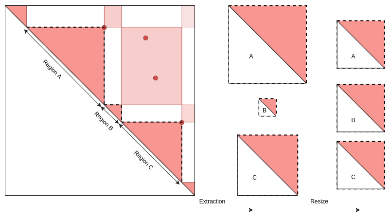
Regions defined with GInteraction object or Pairs of GRanges

The region’s start is defined by the center of the first element and the region’s end by the center of the second element.

interactions_RFmatrix_ctrl.lst  <- ExtractSubmatrix(
    genomicFeature         = interactions.gni,
    hicLst        = HiC_Ctrl.cmx_lst,
    hicResolution            = NULL,
    referencePoint = "rf",
    matriceDim     = 101
    )

Regions defined with GRanges

The regions are directly defined by the ranges of GRanges object.

domains_RFmatrix.lst <- ExtractSubmatrix(
    genomicFeature         = TADs_Domains.gnr,
    hicLst        = HiC_Ctrl.cmx_lst,
    referencePoint = "rf",
    matriceDim     = 101,
    cores          = 1,
    verbose        = FALSE
    )

Case 3: Interactions along the chromosome axis.

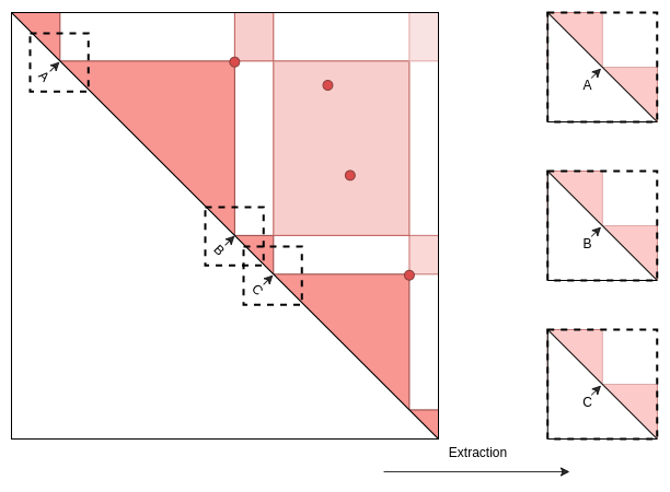
Example to analyse interactions in the context of TADs:

Step 1: generate a GRanges object of TAD boundaries by concatenating starts and ends of TADs.

domains_Border.gnr <- c(
        GenomicRanges::resize(TADs_Domains.gnr, 1, "start"),
        GenomicRanges::resize(TADs_Domains.gnr, 1,  "end" )
) |>
sort()

Step 2: Filter and reduce TAD boundaries GRanges object according to HiC resolution (binSize) + Store TAD names.

domains_Border_Bin.gnr <- BinGRanges(
    gRange  = domains_Border.gnr,
    binSize = binSize,
    verbose = FALSE
    )
domains_Border_Bin.gnr$subname <- domains_Border_Bin.gnr$name
domains_Border_Bin.gnr$name    <- domains_Border_Bin.gnr$bin

domains_Border_Bin.gnr

View

seq	start	end	strand	name	score	class	bin	subname
2L	70001	75000	*	2L:15	3	active	2L:15	Tad_1
2L	90001	95000	*	2L:19	3, 8	active	2L:19	Tad_1, Tad_2
2L	100001	105000	*	2L:21	8	active	2L:21	Tad_2, Tad_3

Step 3: This defines a GRanges object. In the folowing examples, the same information is needed in a GInteraction object class.

domains_Border_Bin.gni <- 
    InteractionSet::GInteractions(
        domains_Border_Bin.gnr,domains_Border_Bin.gnr)

View

First								Second
seq	start	end	name	score	class	bin	subname	seq	start	end	name	score	class	bin	subname
2L	70001	75000	2L:15	3	active	2L:15	Tad_1	2L	70001	75000	2L:15	active	3	2L:15	Tad_1
2L	90001	95000	2L:19	3, 8	active	2L:19	Tad_1, Tad_2	2L	90001	95000	2L:19	active	3, 8	2L:19	Tad_1, Tad_2
2L	100001	105000	2L:21	8	active	2L:21	Tad_2, Tad_3	2L	100001	105000	2L:21	active	8	2L:21	Tad_2, Tad_3

Ponctual interactions defined with GRanges

Here the start and the end of each ranges are in a same bin.

border_PFmatrix.lst <- ExtractSubmatrix(
    genomicFeature         = domains_Border_Bin.gnr,
    hicLst        = HiC_Ctrl.cmx_lst,
    referencePoint = "pf",
    matriceDim     = 101
)

Ponctual interactions defined with GInteractions

Here the first (blue on scheme) and the second (red on scheme) elements are the same.

border_PFmatrix.lst <- ExtractSubmatrix(
    genomicFeature         = domains_Border_Bin.gni,
    hicLst        = HiC_Ctrl.cmx_lst,
    referencePoint = "pf",
    matriceDim     = 101
)

Tips

If hicResolution is NULL, the function will atuomatically use the resolution of the hicLst attributes.
referencePoint is automatically set as “pf” if every anchors and baits are on the same bin (see examples).

Filtrations

The modularity of the workflow allows the user to filter interactions, pairs or extracted submatrices at any step of the analysis. FilterInteractions function takes as input either a GInteraction object or a list of submatrices, and a list of targets of choice and a selectionFunction defining how targets are filtered.

Target list definition:

Target list must be defined by a named list corresponding to the same names of each element and correspond to the column of the GInteraction (or the attributes “interactions” of the matrices to be filtered). Then each element must be a character list to match this column or a function that will test each row in the column and return a bolean.

structureTarget.lst <- list(
    first_colname_of_GInteraction  = c("value"),
    second_colname_of_GInteraction = function(eachElement){
        min_th<value && value<max_th}
    )

Interactions, pairs or extracted submatrices are filtered by metadata elements from GRanges objects used in SearchPairs. Those metadata are stored in the attributes of the list of submatrices that are accessible as follow:

attributes(interactions_RFmatrix_ctrl.lst)$interactions
names(S4Vectors::mcols(attributes(interactions_RFmatrix_ctrl.lst)$interactions))

View

Ranges						Metadata
First			Second			Interaction					Anchor					Bait
seq	start	end	seq	start	end	name	constraint	distance	orientation	submatrix.name	name	bin	Beaf.name	Beaf.score	Beaf.bln	name	bin	Tss.name	Tss.class	Tss.bln
2L	120001	125000	2L	105001	110000	2L:25_2L:22	Tad_3	15000	FALSE	2L:22_2L:25	2L:25:Tad_3	2L:25	Beaf32_15	484	TRUE	2L:22:Tad_3	2L:22	FBgn0026….	active	TRUE
2L	470001	475000	2L	420001	425000	2L:95_2L:85	Tad_17	50000	FALSE	2L:85_2L:95	2L:95:Tad_17	2L:95	Beaf32_62	37	TRUE	2L:85:Tad_17	2L:85	FBgn0031253	active	TRUE
2L	470001	475000	2L	450001	455000	2L:95_2L:91	Tad_17	20000	FALSE	2L:91_2L:95	2L:95:Tad_17	2L:95	Beaf32_62	37	TRUE	2L:91:Tad_17	2L:91	FBgn0015924	active	TRUE
2L	2490001	2495000	2L	2530001	2535000	2L:499_2L:507	Tad_64	40000	TRUE	2L:499_2L:507	2L:499:Tad_64	2L:499	Beaf32_204	231	TRUE	2L:507:Tad_64	2L:507	FBgn0264943	inactive	TRUE
2L	2675001	2680000	2L	2650001	2655000	2L:536_2L:531	Tad_67	25000	FALSE	2L:531_2L:536	2L:536:Tad_67	2L:536	Beaf32_210	124	TRUE	2L:531:Tad_67	2L:531	FBgn0031442	inactive	TRUE
2L	2800001	2805000	2L	2770001	2775000	2L:561_2L:555	Tad_70	30000	FALSE	2L:555_2L:561	2L:561:Tad_70	2L:561	Beaf32_227	185	TRUE	2L:555:Tad_70	2L:555	FBgn0019….	active	TRUE
2L	2805001	2810000	2L	2770001	2775000	2L:562_2L:555	Tad_70	35000	FALSE	2L:555_2L:562	2L:562:Tad_70	2L:562	Beaf32_227	185	TRUE	2L:555:Tad_70	2L:555	FBgn0019….	active	TRUE
2L	2975001	2980000	2L	2990001	2995000	2L:596_2L:599	Tad_76	15000	TRUE	2L:596_2L:599	2L:596:Tad_76	2L:596	Beaf32_244	98	TRUE	2L:599:Tad_76	2L:599	FBgn0025681	active	TRUE
2L	3345001	3350000	2L	3330001	3335000	2L:670_2L:667	Tad_86	15000	FALSE	2L:667_2L:670	2L:670:Tad_86	2L:670	Beaf32_2….	179	TRUE	2L:667:Tad_86	2L:667	FBgn0031523	inactive	TRUE
2L	3350001	3355000	2L	3330001	3335000	2L:671_2L:667	Tad_86	20000	FALSE	2L:667_2L:671	2L:671:Tad_86	2L:671	Beaf32_281	100	TRUE	2L:667:Tad_86	2L:667	FBgn0031523	inactive	TRUE

Example of target list:

In this example, Pairs will be filtered on anchor.Beaf.name, bait.Tss.name, name (which correponds to the submatrix IDs) and distance. The aim of the example is to filter Pairs or submatrices that have:

“Beaf32_62” and “Beaf32_204” in anchor.Beaf.name
“FBgn0015924” and “FBgn0264943” in bait.Tss.name
distance exactly equal to 20000 or 40000 And to exclude Pairs or submatrices that have:
“2L:25_2L:22” in name

targets <- list(
    anchor.Beaf.name = c("Beaf32_62","Beaf32_204"),
    bait.Tss.name    = c("FBgn0015924","FBgn0264943"),
    name             = c("2L:25_2L:22"),
    distance         = function(columnElement){
        return(20000==columnElement || columnElement == 40000)
        }
    )

Selection Function definition:

The selectionFunction defines which operations (union(), intersect(), setdiff()…) are used to filter the set of Pairs with target elements. For more examples, see Selection function tips and examples section.

Example of selectionFunction according to the example target

Following the example case defined in targets

selectionFun = function(){
    Reduce(intersect, list(anchor.Beaf.name, bait.Tss.name ,distance) ) |>
    setdiff(name)
    }

Filtration with selection

Example of GInteraction object filtration

With a GInteraction object as input, FilterInteractions will return the indices of filtered elements.

With the targets and selectionFun defined above:

FilterInteractions(
    genomicInteractions = 
        attributes(interactions_RFmatrix_ctrl.lst)$interactions,
    targets        = targets,
    selectionFun     = selectionFun
    )
#> [1] 3 4

Example of Matrices list filtration

With a matrices list as input, FilterInteractions will return the filtered matrices list, with updated attributes.

With the targets and selectionFun defined above:

filtred_interactions_RFmatrix_ctrl.lst <- FilterInteractions(
    matrices  = interactions_RFmatrix_ctrl.lst,
    targets    = targets,
    selectionFun = selectionFun
    )

Specific case 1: Only one target (and therefore no selection needed)

For example, to filter the top 100 first elements, select the top 100 first names

first100_targets = list(
    submatrix.name = names(interactions_RFmatrix_ctrl.lst)[1:100]
    )

GInteraction filtration

FilterInteractions(
    genomicInteractions = 
        attributes(interactions_RFmatrix_ctrl.lst)$interactions,
    targets        = first100_targets,
    selectionFun     = NULL
    ) |> head()
#> submatrix.name1 submatrix.name2 submatrix.name3 submatrix.name4 submatrix.name5 
#>               1               2               3               4               5 
#> submatrix.name6 
#>               6

Matrices list filtration

first100_interactions_RFmatrix_ctrl.lst <- FilterInteractions(
    matrices  = interactions_RFmatrix_ctrl.lst,
    targets    = first100_targets,
    selectionFun = NULL
    )
attributes(first100_interactions_RFmatrix_ctrl.lst)$interactions
#> GInteractions object with 100 interactions and 15 metadata columns:
#>                   seqnames1           ranges1     seqnames2           ranges2 |
#>                       <Rle>         <IRanges>         <Rle>         <IRanges> |
#>       2L:25_2L:22        2L     120001-125000 ---        2L     105001-110000 |
#>       2L:95_2L:85        2L     470001-475000 ---        2L     420001-425000 |
#>       2L:95_2L:91        2L     470001-475000 ---        2L     450001-455000 |
#>     2L:499_2L:507        2L   2490001-2495000 ---        2L   2530001-2535000 |
#>     2L:536_2L:531        2L   2675001-2680000 ---        2L   2650001-2655000 |
#>               ...       ...               ... ...       ...               ... .
#>   2L:4313_2L:4299        2L 21560001-21565000 ---        2L 21490001-21495000 |
#>   2L:4315_2L:4299        2L 21570001-21575000 ---        2L 21490001-21495000 |
#>   2L:4312_2L:4305        2L 21555001-21560000 ---        2L 21520001-21525000 |
#>   2L:4313_2L:4305        2L 21560001-21565000 ---        2L 21520001-21525000 |
#>   2L:4315_2L:4305        2L 21570001-21575000 ---        2L 21520001-21525000 |
#>                              name  constraint  distance orientation
#>                       <character> <character> <integer>   <logical>
#>       2L:25_2L:22     2L:25_2L:22       Tad_3     15000       FALSE
#>       2L:95_2L:85     2L:95_2L:85      Tad_17     50000       FALSE
#>       2L:95_2L:91     2L:95_2L:91      Tad_17     20000       FALSE
#>     2L:499_2L:507   2L:499_2L:507      Tad_64     40000        TRUE
#>     2L:536_2L:531   2L:536_2L:531      Tad_67     25000       FALSE
#>               ...             ...         ...       ...         ...
#>   2L:4313_2L:4299 2L:4313_2L:4299     Tad_486     70000       FALSE
#>   2L:4315_2L:4299 2L:4315_2L:4299     Tad_486     80000       FALSE
#>   2L:4312_2L:4305 2L:4312_2L:4305     Tad_486     35000       FALSE
#>   2L:4313_2L:4305 2L:4313_2L:4305     Tad_486     40000       FALSE
#>   2L:4315_2L:4305 2L:4315_2L:4305     Tad_486     50000       FALSE
#>                    submatrix.name  anchor.bin     anchor.name    bait.bin
#>                       <character> <character>     <character> <character>
#>       2L:25_2L:22     2L:22_2L:25       2L:25     2L:25:Tad_3       2L:22
#>       2L:95_2L:85     2L:85_2L:95       2L:95    2L:95:Tad_17       2L:85
#>       2L:95_2L:91     2L:91_2L:95       2L:95    2L:95:Tad_17       2L:91
#>     2L:499_2L:507   2L:499_2L:507      2L:499   2L:499:Tad_64      2L:507
#>     2L:536_2L:531   2L:531_2L:536      2L:536   2L:536:Tad_67      2L:531
#>               ...             ...         ...             ...         ...
#>   2L:4313_2L:4299 2L:4299_2L:4313     2L:4313 2L:4313:Tad_486     2L:4299
#>   2L:4315_2L:4299 2L:4299_2L:4315     2L:4315 2L:4315:Tad_486     2L:4299
#>   2L:4312_2L:4305 2L:4305_2L:4312     2L:4312 2L:4312:Tad_486     2L:4305
#>   2L:4313_2L:4305 2L:4305_2L:4313     2L:4313 2L:4313:Tad_486     2L:4305
#>   2L:4315_2L:4305 2L:4305_2L:4315     2L:4315 2L:4315:Tad_486     2L:4305
#>                         bait.name anchor.Beaf.score anchor.Beaf.name
#>                       <character>         <numeric>           <list>
#>       2L:25_2L:22     2L:22:Tad_3               484        Beaf32_15
#>       2L:95_2L:85    2L:85:Tad_17                37        Beaf32_62
#>       2L:95_2L:91    2L:91:Tad_17                37        Beaf32_62
#>     2L:499_2L:507   2L:507:Tad_64               231       Beaf32_204
#>     2L:536_2L:531   2L:531:Tad_67               124       Beaf32_210
#>               ...             ...               ...              ...
#>   2L:4313_2L:4299 2L:4299:Tad_486               748      Beaf32_1348
#>   2L:4315_2L:4299 2L:4299:Tad_486               529      Beaf32_1349
#>   2L:4312_2L:4305 2L:4305:Tad_486               748      Beaf32_1348
#>   2L:4313_2L:4305 2L:4305:Tad_486               748      Beaf32_1348
#>   2L:4315_2L:4305 2L:4305:Tad_486               529      Beaf32_1349
#>                   anchor.Beaf.bln bait.Tss.class           bait.Tss.name
#>                         <logical>         <list>                  <list>
#>       2L:25_2L:22            TRUE         active FBgn0026787,FBgn0005278
#>       2L:95_2L:85            TRUE         active             FBgn0031253
#>       2L:95_2L:91            TRUE         active             FBgn0015924
#>     2L:499_2L:507            TRUE       inactive             FBgn0264943
#>     2L:536_2L:531            TRUE       inactive             FBgn0031442
#>               ...             ...            ...                     ...
#>   2L:4313_2L:4299            TRUE       inactive             FBgn0053837
#>   2L:4315_2L:4299            TRUE       inactive             FBgn0053837
#>   2L:4312_2L:4305            TRUE       inactive             FBgn0053873
#>   2L:4313_2L:4305            TRUE       inactive             FBgn0053873
#>   2L:4315_2L:4305            TRUE       inactive             FBgn0053873
#>                   bait.Tss.bln
#>                      <logical>
#>       2L:25_2L:22         TRUE
#>       2L:95_2L:85         TRUE
#>       2L:95_2L:91         TRUE
#>     2L:499_2L:507         TRUE
#>     2L:536_2L:531         TRUE
#>               ...          ...
#>   2L:4313_2L:4299         TRUE
#>   2L:4315_2L:4299         TRUE
#>   2L:4312_2L:4305         TRUE
#>   2L:4313_2L:4305         TRUE
#>   2L:4315_2L:4305         TRUE
#>   -------
#>   regions: 335 ranges and 0 metadata columns
#>   seqinfo: 2 sequences from an unspecified genome

Warning! A selection of some matrices removes attributes.

attributes(interactions_RFmatrix_ctrl.lst[1:20])$interactions
#> NULL

Specific case 2: Sampling

nSample.num = 3
set.seed(123)
targets = list(name=sample(
    attributes(interactions_RFmatrix_ctrl.lst)$interactions$name,nSample.num))

GInteraction sampling

FilterInteractions(
    genomicInteractions = 
        attributes(interactions_RFmatrix_ctrl.lst)$interactions,
    targets        = targets,
    selectionFun     = NULL
    )
#> name1 name2 name3 
#>    14    50   118

Matrices list sampling

sampled_interactions_RFmatrix_ctrl.lst <- FilterInteractions(
    matrices  = interactions_RFmatrix_ctrl.lst,
    targets    = targets,
    selectionFun = NULL
    )
attributes(sampled_interactions_RFmatrix_ctrl.lst)$interactions
#> GInteractions object with 3 interactions and 15 metadata columns:
#>                   seqnames1           ranges1     seqnames2           ranges2 |
#>                       <Rle>         <IRanges>         <Rle>         <IRanges> |
#>   2L:1012_2L:1015        2L   5055001-5060000 ---        2L   5070001-5075000 |
#>   2L:3002_2L:2978        2L 15005001-15010000 ---        2L 14885001-14890000 |
#>   2R:1824_2R:1820        2R   9115001-9120000 ---        2R   9095001-9100000 |
#>                              name  constraint  distance orientation
#>                       <character> <character> <integer>   <logical>
#>   2L:1012_2L:1015 2L:1012_2L:1015     Tad_132     15000        TRUE
#>   2L:3002_2L:2978 2L:3002_2L:2978     Tad_356    120000       FALSE
#>   2R:1824_2R:1820 2R:1824_2R:1820     Tad_608     20000       FALSE
#>                    submatrix.name  anchor.bin     anchor.name    bait.bin
#>                       <character> <character>     <character> <character>
#>   2L:1012_2L:1015 2L:1012_2L:1015     2L:1012 2L:1012:Tad_132     2L:1015
#>   2L:3002_2L:2978 2L:2978_2L:3002     2L:3002 2L:3002:Tad_356     2L:2978
#>   2R:1824_2R:1820 2R:1820_2R:1824     2R:1824 2R:1824:Tad_608     2R:1820
#>                         bait.name anchor.Beaf.score      anchor.Beaf.name
#>                       <character>         <numeric>                <list>
#>   2L:1012_2L:1015 2L:1015:Tad_132               660 Beaf32_374,Beaf32_375
#>   2L:3002_2L:2978 2L:2978:Tad_356                49           Beaf32_1001
#>   2R:1824_2R:1820 2R:1820:Tad_608               977           Beaf32_1734
#>                   anchor.Beaf.bln bait.Tss.class bait.Tss.name bait.Tss.bln
#>                         <logical>         <list>        <list>    <logical>
#>   2L:1012_2L:1015            TRUE         active   FBgn0261608         TRUE
#>   2L:3002_2L:2978            TRUE       inactive   FBgn0266840         TRUE
#>   2R:1824_2R:1820            TRUE         active   FBgn0082927         TRUE
#>   -------
#>   regions: 335 ranges and 0 metadata columns
#>   seqinfo: 2 sequences from an unspecified genome

Specific case 3: Filtration without selectionFunction

Without any selectionFunction, FilterInteractions will return all indices corresponding to each target in the list. Then, the indices of interest can be selected in a second step. For the examples we take the folowing targets:

targets <- list(
    anchor.Beaf.name = c("Beaf32_8","Beaf32_15"),
    bait.Tss.name    = c("FBgn0031214","FBgn0005278"),
    name             = c("2L:74_2L:77"),
    distance         = function(columnElement){
        return(14000==columnElement || columnElement == 3000)
        }
    )

GInteraction filtration

FilterInteractions(
    genomicInteractions = 
        attributes(interactions_RFmatrix_ctrl.lst)$interactions,
    targets        = targets,
    selectionFun     = NULL
    ) |> str()
#> List of 4
#>  $ anchor.Beaf.name: int 1
#>  $ bait.Tss.name   : int 1
#>  $ name            : int(0) 
#>  $ distance        : int(0)

Matrices list filtration

FilterInteractions(
    matrices      = interactions_RFmatrix_ctrl.lst,
    targets        = targets,
    selectionFun     = NULL
    ) |>
str()
#> List of 4
#>  $ anchor.Beaf.name: int 1
#>  $ bait.Tss.name   : int 1
#>  $ name            : int(0) 
#>  $ distance        : int(0)

Tips

Filter a GInteraction object allows to intersect the selected index.
Filter a matrices list without selection is better than filter the interaction attributes of the matrices list

Selection function tips and examples:

a <- c("A","B","D","G")
b <- c("E","B","C","G")
c <- c("A","F","C","G")

What is common to A, B and C

Reduce(intersect, list(a,b,c)) |> sort()
#> [1] "G"

intersect(a,b) |> intersect(c) |> sort()
#> [1] "G"

What is in A and/or B and/or C

Reduce(union, list(a,b,c)) |> sort()
#> [1] "A" "B" "C" "D" "E" "F" "G"

union(a,b) |> union(c) |> sort()
#> [1] "A" "B" "C" "D" "E" "F" "G"

What is only in A

Reduce(setdiff,list(a,b,c)) |> sort()
#> [1] "D"

setdiff(a,b) |> setdiff(c) |> sort()
#> [1] "D"

What is common in A with B, and not in C

intersect(a,b) |> setdiff(c) |> sort()
#> [1] "B"

What is common in A with B, plus all that is present in C

intersect(a,b) |> union(c) |> sort()
#> [1] "A" "B" "C" "F" "G"

What is common in C with all elements present in A and B

union(a,b) |> intersect(c) |> sort()
#> [1] "A" "C" "G"

Everything that is present in A and B but not in C

union(a,b) |> setdiff(c) |> sort()
#> [1] "B" "D" "E"

What is present only once

d <- c(a,b,c)
setdiff(d,d[duplicated(d)]) |> sort()
#> [1] "D" "E" "F"

Orientation

ExtractSubmatrix returns submatrices orientated according to 5’->3’ orientation of the chromosome. In the case of heterotypic or asymetric pairs (anchor != bait), anchors and baits are thus mixed on Y and X axis of the matrices.

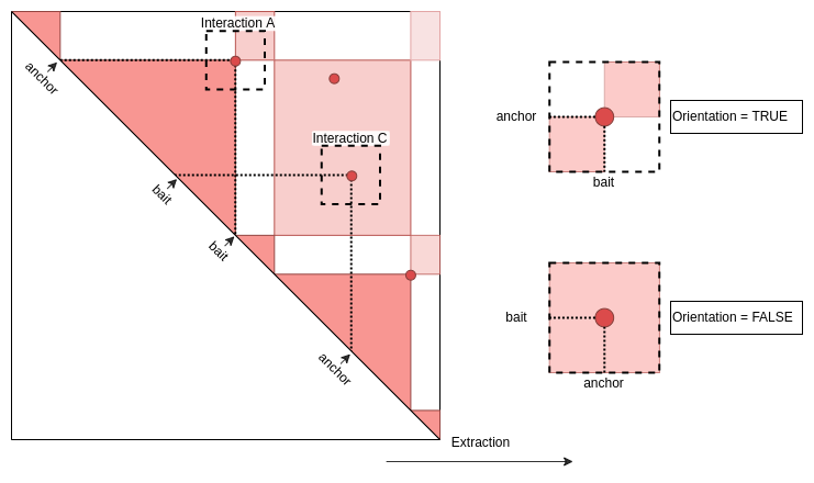
OrientateMatrix function allows to force all matrices to be orientated in a way that anchors will be systematically on Y axis and baits on X axis.

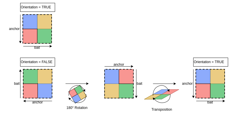
Information about the orientation

# mcols(attributes(
    # first100_interactions_RFmatrix_ctrl.lst)$interactions)$orientation

The 13th matrice is well oriented, i.e. the anchor Beaf is in Y axis and the bait TSS in X axis
The 14th matrice is not well oriented, i.e. the bait TSS is in Y axis and the anchor Beaf in X axis

Orientation on matrices list

oriented_first100_interactions_RFmatrix_ctrl.lst <- 
    OrientateMatrix(first100_interactions_RFmatrix_ctrl.lst)
#> 69 matrices are oriented

Orientation of one matrix only.

Warning This procedure force orientation even if not needed.

orientedMatrix.mtx <- 
    OrientateMatrix(first100_interactions_RFmatrix_ctrl.lst[[1]])

Prepare matrices list

PrepareMtxList can be used to perform operations on the matrices list. This function prepares the matrices list by performing a per matrix operation by transforming values. For example values can be quantilized inorder to rank local interactions and highlight on the contacts with the highest values. This function can also be used to correct orientations, just as OrientateMatrix. The reason for giving access for the user to this originally hidden function is to have a uniformly prepared matrices list for both quantifications and visualisations.

oriented_quantiled_first100_interactions_RFmatrix_ctrl.lst <- 
    PrepareMtxList(
        first100_interactions_RFmatrix_ctrl.lst,
        transFun = 'quantile',
        orientate = TRUE)
#> 69 matrices are oriented

oriented_first100_interactions_RFmatrix_ctrl.lst <- 
    PrepareMtxList(
        first100_interactions_RFmatrix_ctrl.lst,
        orientate = TRUE)
#> 69 matrices are oriented

Quantifications

GetQuantif function takes as input a list of submatrices and returns a vector of contact frequencies in a given typeof regions where these contacts are computed with a function.

Basic quantifications

The GetQuantif function extracts per submatrix the average values of the 3*3 central pixels by default (see GetQuantif).

area: The region where the contacts values are extracted in each matrix.
operation The function that is done on extracted values for each matrix.

Example: Average of the values in the centered 3x3 square.

center.num <- GetQuantif(
    matrices  = oriented_first100_interactions_RFmatrix_ctrl.lst,
    areaFun      = "center",
    operationFun = "mean"
    )

Custom functions

The GetQuantif function also takes custom area and operation in parameter.

area: function defining on which submatrix coordinates the values are extracted in each matrices.
operation function defining which operation is done on extracted values for each matrices.

Example: Interactions values on the matrice.mtx[33:35,67:69] area, averaged after removing all zeros.

GetQuantif(
    matrices  = oriented_first100_interactions_RFmatrix_ctrl.lst,
    areaFun      = function(matrice.mtx){matrice.mtx[33:35,67:69]},
    operationFun = function(area.mtx){
        area.mtx[which(area.mtx==0)]<-NA;
        return(mean(area.mtx,na.rm=TRUE))
        }
    ) |>
c() |>
unlist() |>
head()
#>   2L:25_2L:22   2L:95_2L:85   2L:95_2L:91 2L:499_2L:507 2L:536_2L:531 
#>     1.2652268     1.0275631     1.8478690     0.8648371     1.1975185 
#> 2L:561_2L:555 
#>     1.6126441

Particular cases:

Values naming

By default, returned values are named with submatrix ID. If varName is set with an element metadata column name from GInteraction attributes, values are returned values are named according to this element.

Example: Named quantifications with anchor.Beaf.name

namedCenter.num <- GetQuantif(
    matrices  = oriented_first100_interactions_RFmatrix_ctrl.lst,
    areaFun      = "center",
    operationFun = "mean",
    varName      = "anchor.Beaf.name"
    )

Note that changing submatrix ID for other names can create name duplicates:

Example: The 46th matrix is correspond to two Beaf32 peaks, i.e. it has two anchor.Beaf.name

	name	anchor.Beaf.name
45	2L:2676_2L:2680	Beaf32_950
46	2L:2768_2L:2765	Beaf32_981
47	2L:2971_2L:2977	Beaf32_1000
48	2L:3002_2L:2977	Beaf32_1001
49	2L:2971_2L:2978	Beaf32_1000
50	2L:3002_2L:2978	Beaf32_1001

As a consequence, the value in center.num is duplicated in namedCenter.num

unlist(c(center.num))[45:50]
#> 2L:2676_2L:2680 2L:2768_2L:2765 2L:2971_2L:2977 2L:3002_2L:2977 2L:2971_2L:2978 
#>       0.7318490       0.8071858       0.5238616       0.7522744       0.5438497 
#> 2L:3002_2L:2978 
#>       0.7135216

unlist(c(namedCenter.num))[45:51]
#> Beaf32_378 Beaf32_408 Beaf32_408 Beaf32_408 Beaf32_437 Beaf32_518 Beaf32_521 
#>  1.1762447  1.0476893  0.8868763  0.7318490  0.8071858  0.5238616  0.7522744

Duplicated value index are stored in attributes.

attributes(center.num)$duplicated
#> NULL

attributes(namedCenter.num)$duplicated
#> NULL

One value extraction

GetQuantif(
    matrices  = oriented_first100_interactions_RFmatrix_ctrl.lst,
    areaFun      = function(matrice.mtx){matrice.mtx[5,5]},
    operationFun = function(area.mtx){area.mtx}
    ) |>
head()
#>   2L:25_2L:22   2L:95_2L:85   2L:95_2L:91 2L:499_2L:507 2L:536_2L:531 
#>     1.6036209     1.2231158     1.2129980     0.8516612     0.3858703 
#> 2L:561_2L:555 
#>     0.8043792

Area extraction

GetQuantif(
    matrices  = oriented_first100_interactions_RFmatrix_ctrl.lst,
    areaFun      = function(matrice.mtx){matrice.mtx[4:6,4:6]},
    operationFun = function(area){area}
    ) |>
head()
#>   2L:25_2L:22   2L:95_2L:85   2L:95_2L:91 2L:499_2L:507 2L:536_2L:531 
#>      1.599228            NA            NA      1.716875      1.603621 
#> 2L:561_2L:555 
#>            NA

Tips

If operationFun is NULL then it will return values of the selected region without NA.

GetQuantif(
    matrices  = oriented_first100_interactions_RFmatrix_ctrl.lst,
    areaFun      = function(matrice.mtx){matrice.mtx[4:6,4:6]},
    operationFun = NULL
    ) |>
head()
#>   2L:25_2L:22   2L:95_2L:85   2L:95_2L:91 2L:499_2L:507 2L:536_2L:531 
#>      1.599228      1.716875      1.603621      1.834523      1.731368 
#> 2L:561_2L:555 
#>      1.628212

Aggregations

Aggregation function takes as input a list of submatrices and returns an aggregated matrix using the aggregation function defined by the user.

One sample aggregation

Basic aggregation

Aggregation function has some default aggregation functions like sum, mean or median (see Aggregation)

# rm0 argument can be added to PrepareMtxList to assign NA to 0 values.
oriented_first100_interactions_RFmatrix_ctrl.lst = 
    PrepareMtxList(
        oriented_first100_interactions_RFmatrix_ctrl.lst,
        rm0 = FALSE)
agg_sum.mtx <- Aggregation(
    matrices = oriented_first100_interactions_RFmatrix_ctrl.lst, 
    aggFun      = "sum"
    )

Custom aggregation

Defining a custom aggregation function: example below shows the mean function after removing NA.

agg_mean.mtx <- Aggregation(
    matrices = oriented_first100_interactions_RFmatrix_ctrl.lst,
    aggFun      = function(x){mean(x,na.rm=TRUE)}
    )

Two samples differential aggregation

Aggregation function can take as input two list of submatrices from two samples or conditions and returns a differential aggregated matrix. Two ways to obtain differential aggregation are applied, first is by assessing differences on each individual pairs of submatrices then aggregate the differences; second is by aggregating matrices and assess differences on the aggregated matrices (see examples below).

Preparation of matrices list

Preparation of Control matrices list condition
Filtration

first100_targets = list(
    submatrix.name = names(interactions_RFmatrix_ctrl.lst)[1:100]
    )
first100_interactions_RFmatrix_ctrl.lst <- FilterInteractions(
    matrices  = interactions_RFmatrix_ctrl.lst,
    targets    = first100_targets,
    selectionFun = NULL
    )

Orientation

oriented_first100_interactions_RFmatrix_ctrl.lst <- 
    OrientateMatrix(first100_interactions_RFmatrix_ctrl.lst)

Preparation of second matrices list in Beaf depleted condition. Extraction

interactions_RFmatrix.lst  <- ExtractSubmatrix(
    genomicFeature         = interactions.gni,
    hicLst        = HiC_HS.cmx_lst,
    referencePoint = "rf",
    matriceDim     = 101
    )

Filtration

first100_interactions_RFmatrix.lst <- FilterInteractions(
    matrices  = interactions_RFmatrix.lst,
    targets    = first100_targets,
    selectionFun = NULL
    )

Orientation

oriented_first100_interactions_RFmatrix.lst <- 
    OrientateMatrix(first100_interactions_RFmatrix.lst)
#> 69 matrices are oriented

Aggregate

oriented_first100_interactions_RFmatrix_ctrl.lst = 
    PrepareMtxList(first100_interactions_RFmatrix_ctrl.lst,
        minDist   = NULL,
        maxDist   = NULL,
        rm0       = FALSE,
        orientate = TRUE
)
#> 69 matrices are oriented

oriented_first100_interactions_RFmatrix.lst = 
    PrepareMtxList(first100_interactions_RFmatrix.lst,
        minDist   = NULL,
        maxDist   = NULL,
        rm0       = FALSE,
        orientate = TRUE
)
#> 69 matrices are oriented


diffAggreg.mtx <- Aggregation(
    ctrlMatrices    = oriented_first100_interactions_RFmatrix_ctrl.lst,
    matrices        = oriented_first100_interactions_RFmatrix.lst,
    aggFun             = "mean",
    diffFun            = "substraction",
    scaleCorrection = TRUE,
    correctionArea  =  list(
        i = c(1:30),
        j = c(72:101)
        ),
    statCompare = TRUE)

Tips

On PrepareMtxList function:

PrepareMtxList acts as a one stop function to perform value treatment and orientation correction allowing to have consistent matrices list for both quantification and visualization process to come.
If rm0 is TRUE all zeros in matrices list will be replaced by NA.
It is possible to filter submatrices list by minimal or maximal distance during the aggregation function.
It is possible to orientate submatrices at this point or using OrientateMatrix function.
PrepareMtxList keeps former attributes matrices list and adds new ones:
- totalMatrixNumber: total number of matrices.
- filteredMatrixNumber: number of matrices after distance filtering.
- minimalDistance: minimal distance between anchor and bait.
- maximalDistance: maximal distance between anchor and bait.
- transformationMethod: the function used to perform a per matrix data transformation.
- zeroRemoved: A Boolean that indicates if zeros have been replaced by NA.

On Aggregation function:

When aggregation is performed using one sample only, use either matrices or ctrlMatrices parameters
The statCompare may not be set TRUE every time (due to memory requirement).
Aggregation on one sample keeps former attributes of the matrices list and add new ones:
- aggregationMethod: The function applied to obtain the aggregation.
Aggregation on two samples adds additional attributes:
- correctedFact: The value that is added to the condition to reduce noise. It’s computed as the median difference between condition and control in an background area (e.g upper right corner in matrices).
- matrices: The list of matrices.
  - agg: Aggregation of the condition.
  - aggCtrl: Aggregation of the control.
  - aggCorrected: Aggregation of the condition corrected with correctedFact.
  - aggDelta: the difference between the aggregated matrix of the condition and the aggregated matrix of the control.
  - aggCorrectedDelta: the difference between the aggregated matrix of the condition corrected with correctedFact and the aggregated matrix of the control.

Aggregations plots

Preparation of aggregated matrices

Control aggregation with no orientation

aggreg.mtx <- Aggregation(
        ctrlMatrices=interactions_RFmatrix_ctrl.lst,
        aggFun="mean"
)

Control aggregation with orientation

oriented_interactions_RFmatrix_ctrl.lst <- 
    OrientateMatrix(interactions_RFmatrix_ctrl.lst)
#> 95 matrices are oriented

orientedAggreg.mtx <- Aggregation(
        ctrlMatrices=oriented_interactions_RFmatrix_ctrl.lst,
        aggFun="mean"
)

Differential aggregation

oriented_interactions_RFmatrix.lst <- 
    OrientateMatrix(interactions_RFmatrix.lst)
#> 95 matrices are oriented

diffAggreg.mtx <- Aggregation(
        ctrlMatrices    = oriented_interactions_RFmatrix_ctrl.lst,
        matrices        = oriented_interactions_RFmatrix.lst,
        aggFun          = "mean",
        diffFun         = "log2+1",
        scaleCorrection = TRUE,
        correctionArea  = list( i=c(1:30) , j=c(72:101) ),
        statCompare     = TRUE
)

Plots

Simple aggregation plot:

With no orientation

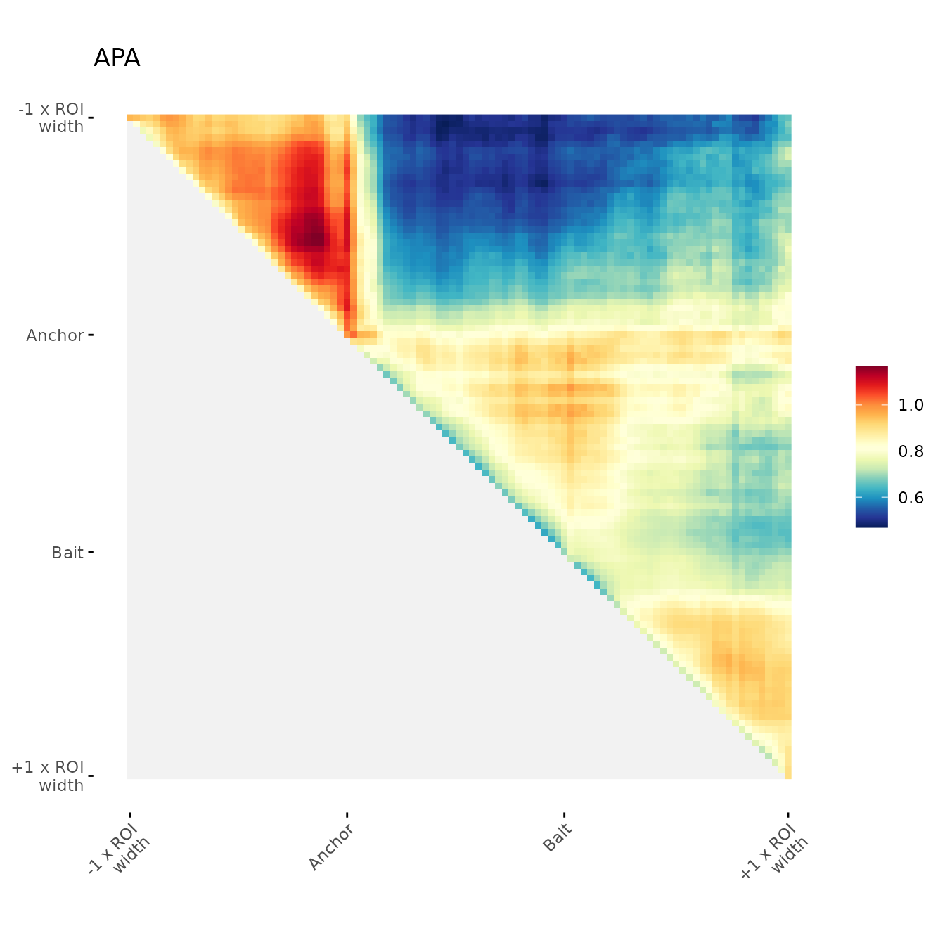
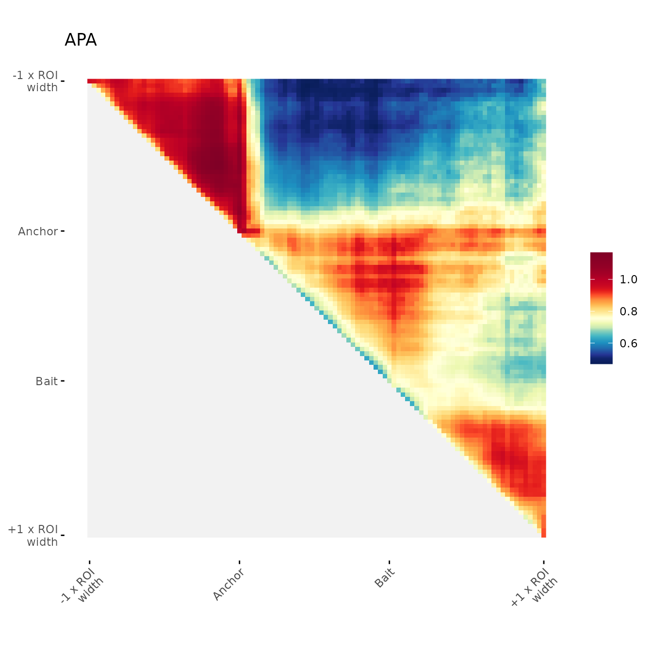
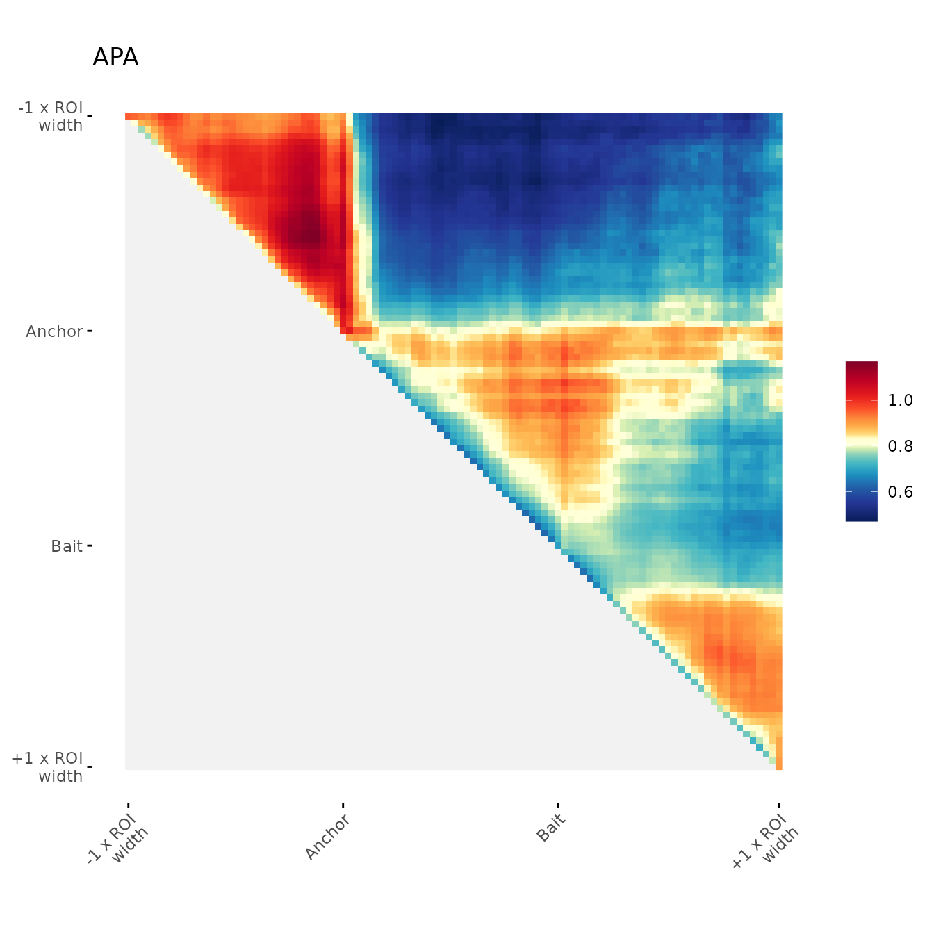
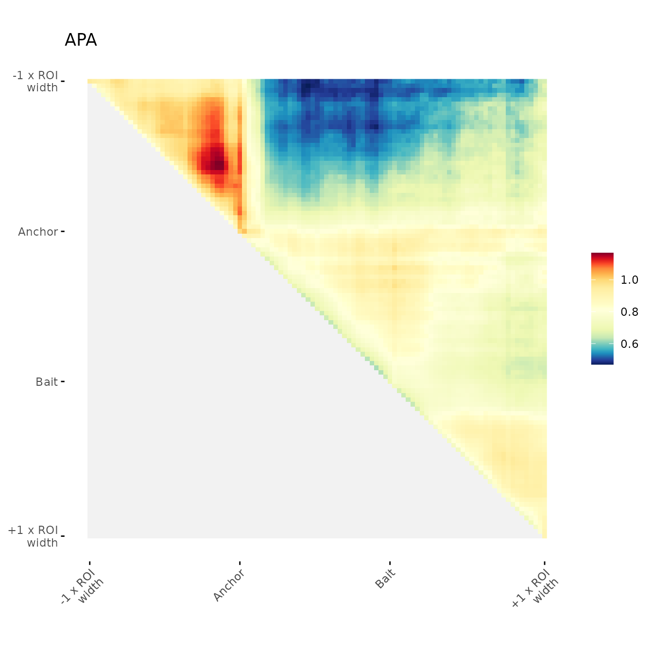
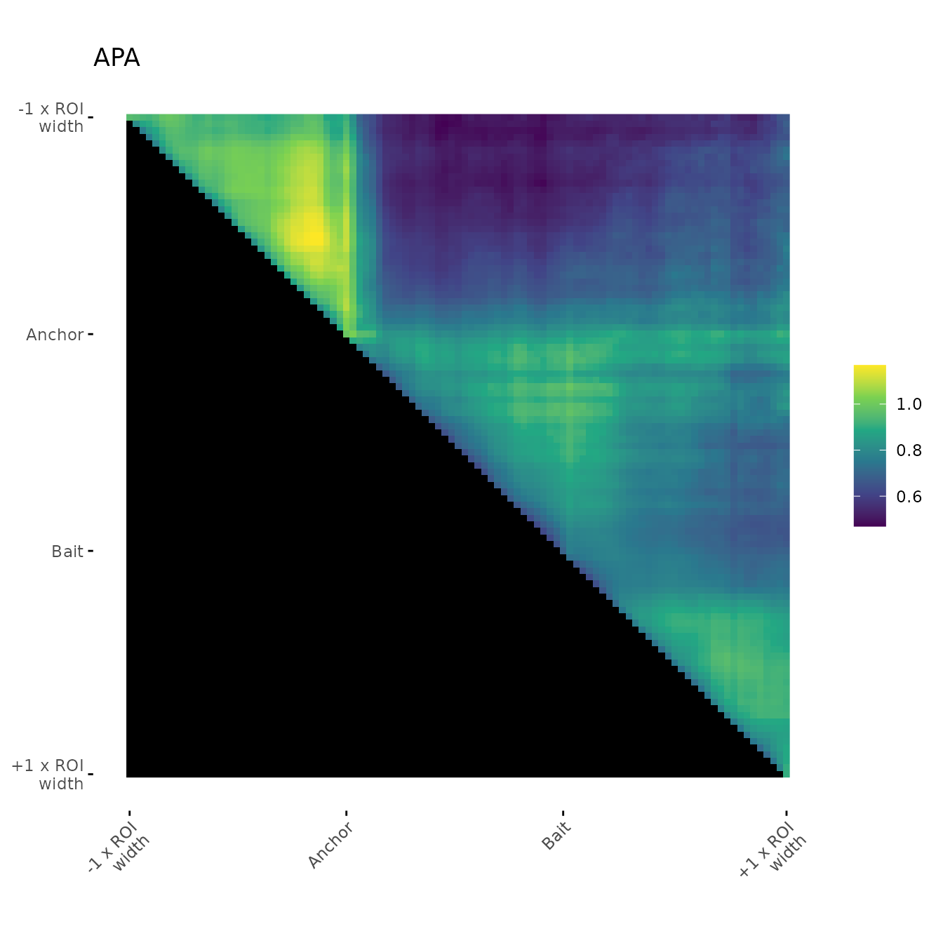
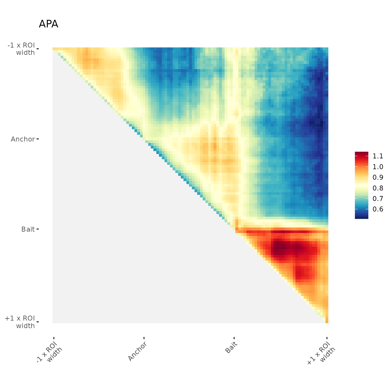
ggAPA function creates a ggplot object (ggplot2::geom_raster)

ggAPA(
        aggregatedMtx   = aggreg.mtx,
        title = "APA"
)

With Orientation

ggAPA(
        aggregatedMtx   = orientedAggreg.mtx,
        title = "APA"
)

Further visualisation parameters:

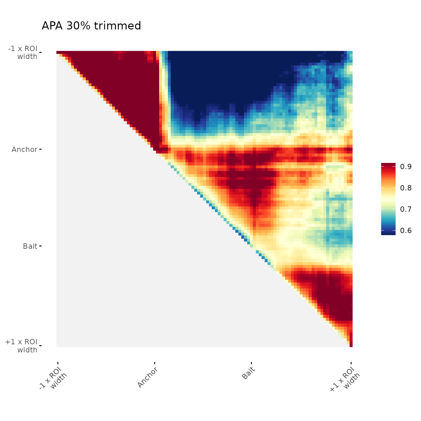
Trimming aggregated values for visualisation:

It is possible to set a specific range of values of the scale, for this remove a percentage of values using upper tail, lower tail or both tails of the distribution.

ggAPA(
        aggregatedMtx      = orientedAggreg.mtx,
        title    = "APA 30% trimmed on upper side",
        trim = 30,
        tails   = "upper"
)
#> Warning in max(unlist(bounds.num_lst[1]), na.rm = TRUE): no non-missing
#> arguments to max; returning -Inf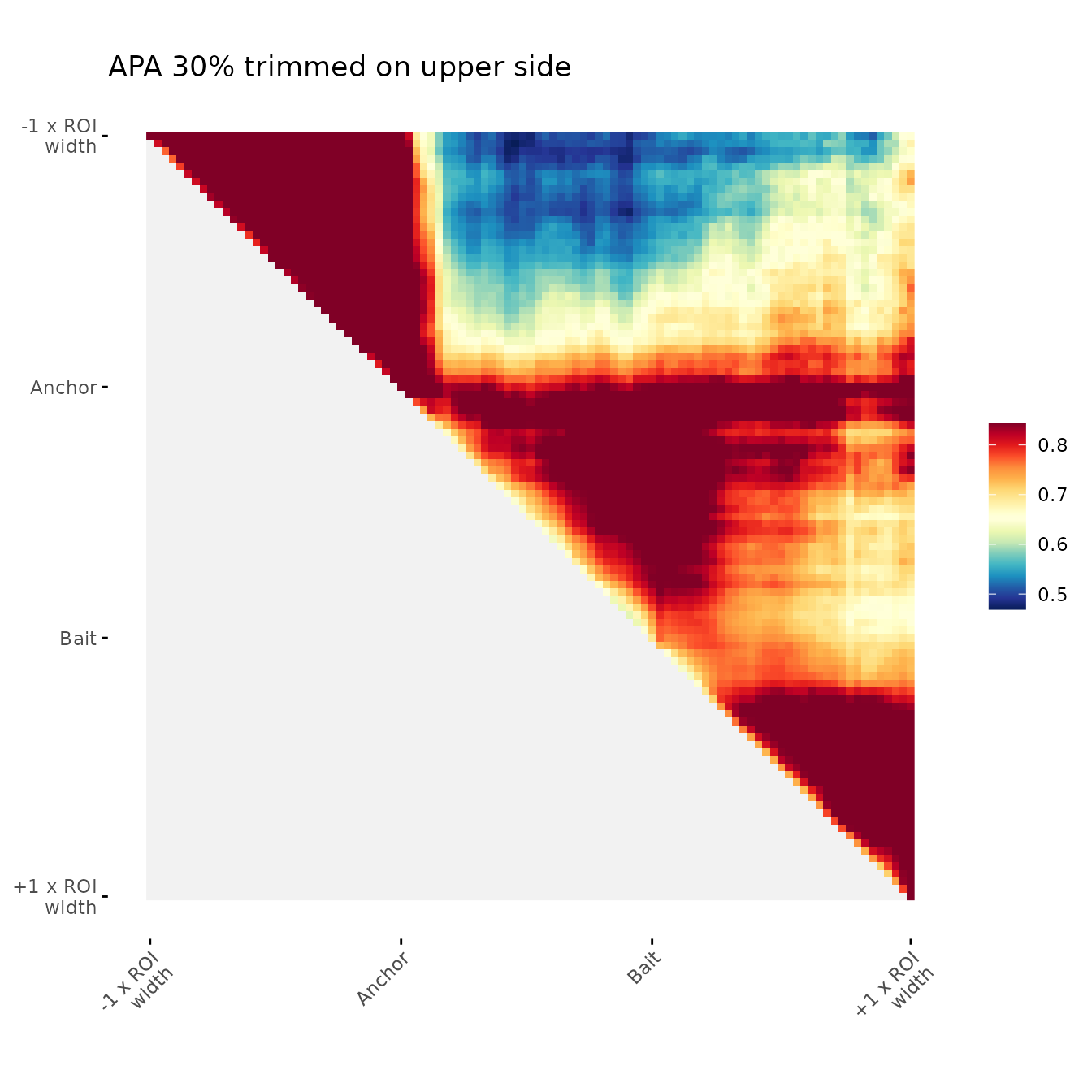

ggAPA(
        aggregatedMtx      = orientedAggreg.mtx,
        title    = "APA 30% trimmed on upper side",
        trim = 30,
        tails   = "lower"
)
#> Warning in min(unlist(bounds.num_lst[2]), na.rm = TRUE): no non-missing
#> arguments to min; returning Inf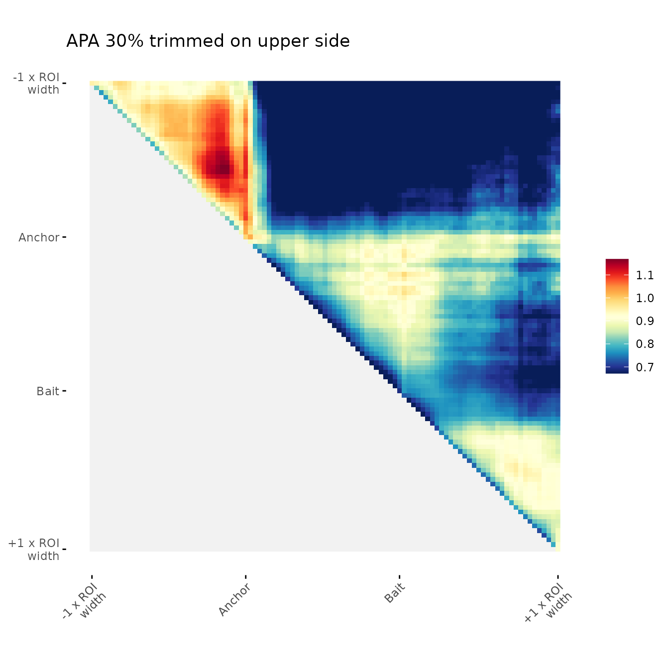

ggAPA(
        aggregatedMtx      = orientedAggreg.mtx,
        title    = "APA 30% trimmed",
        trim = 30,
        tails   = "both"
)

Modifying color scale:

Min and max color scale

Example of user-defined min and max color scale

ggAPA(
        aggregatedMtx         = orientedAggreg.mtx,
        title       = "APA [0-1]",
        colMin = 0,
        colMax = 1
)

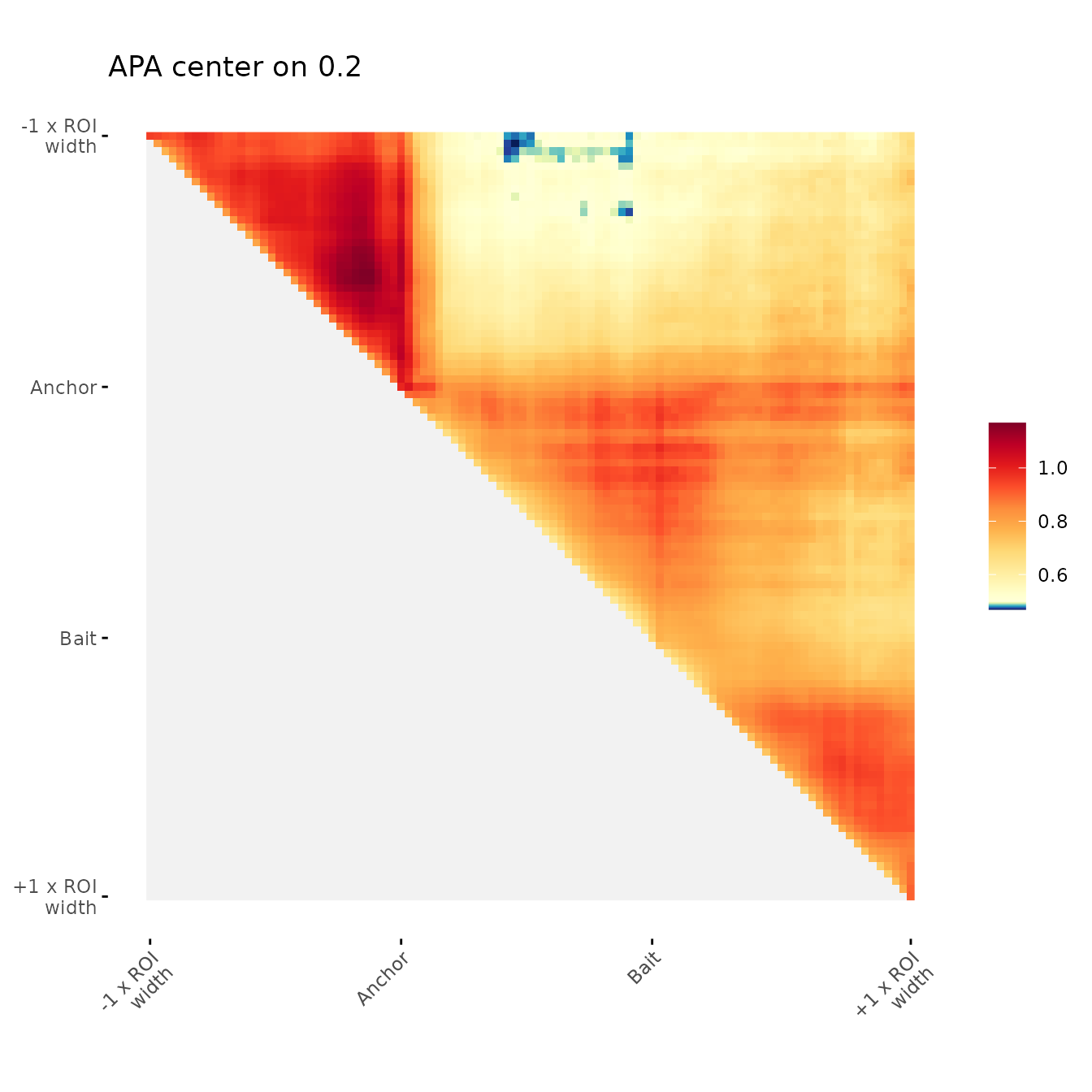
Center color scale

Example of user-defined color scale center

ggAPA(
        aggregatedMtx    = orientedAggreg.mtx,
        title  = "APA center on 0.2",
        colMid = 0.5
)

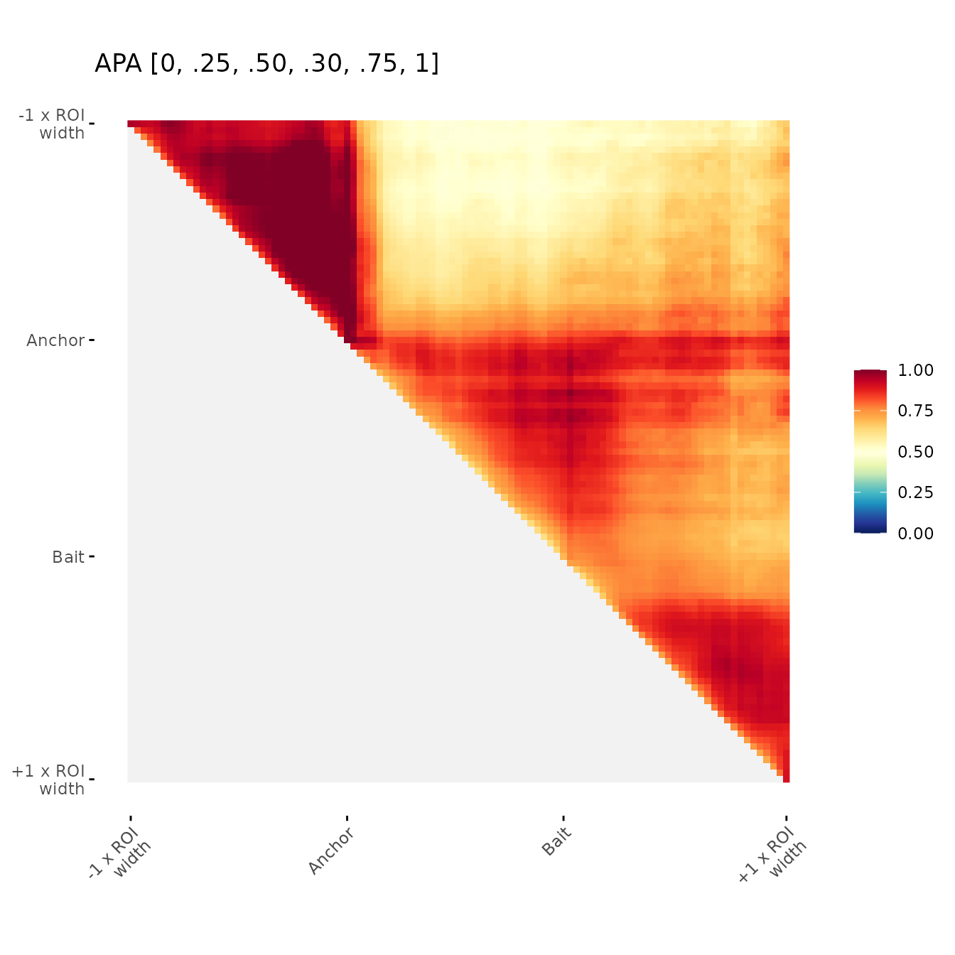
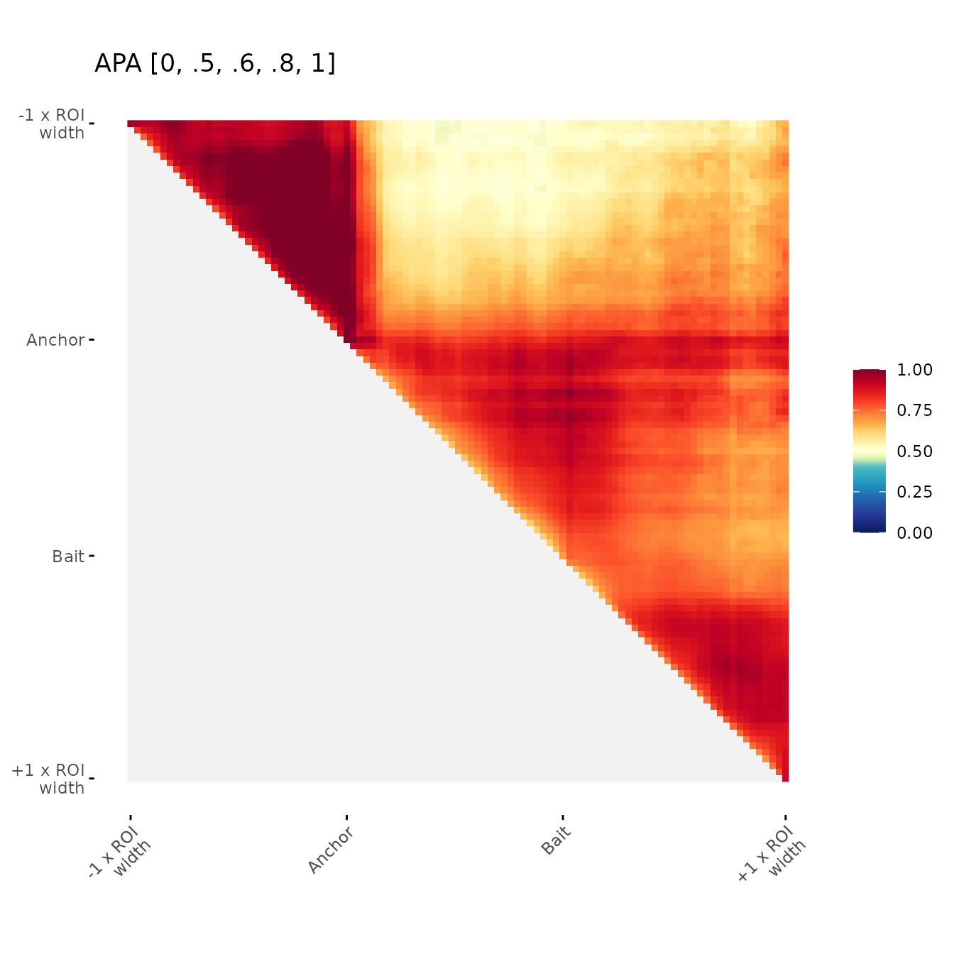
Change color breaks

Examples of user-defined color breaks

ggAPA(
        aggregatedMtx       = orientedAggreg.mtx,
        title     = "APA [0, .25, .50, .30, .75, 1]",
        colBreaks = c(0,0.25,0.5,0.75,1)
)

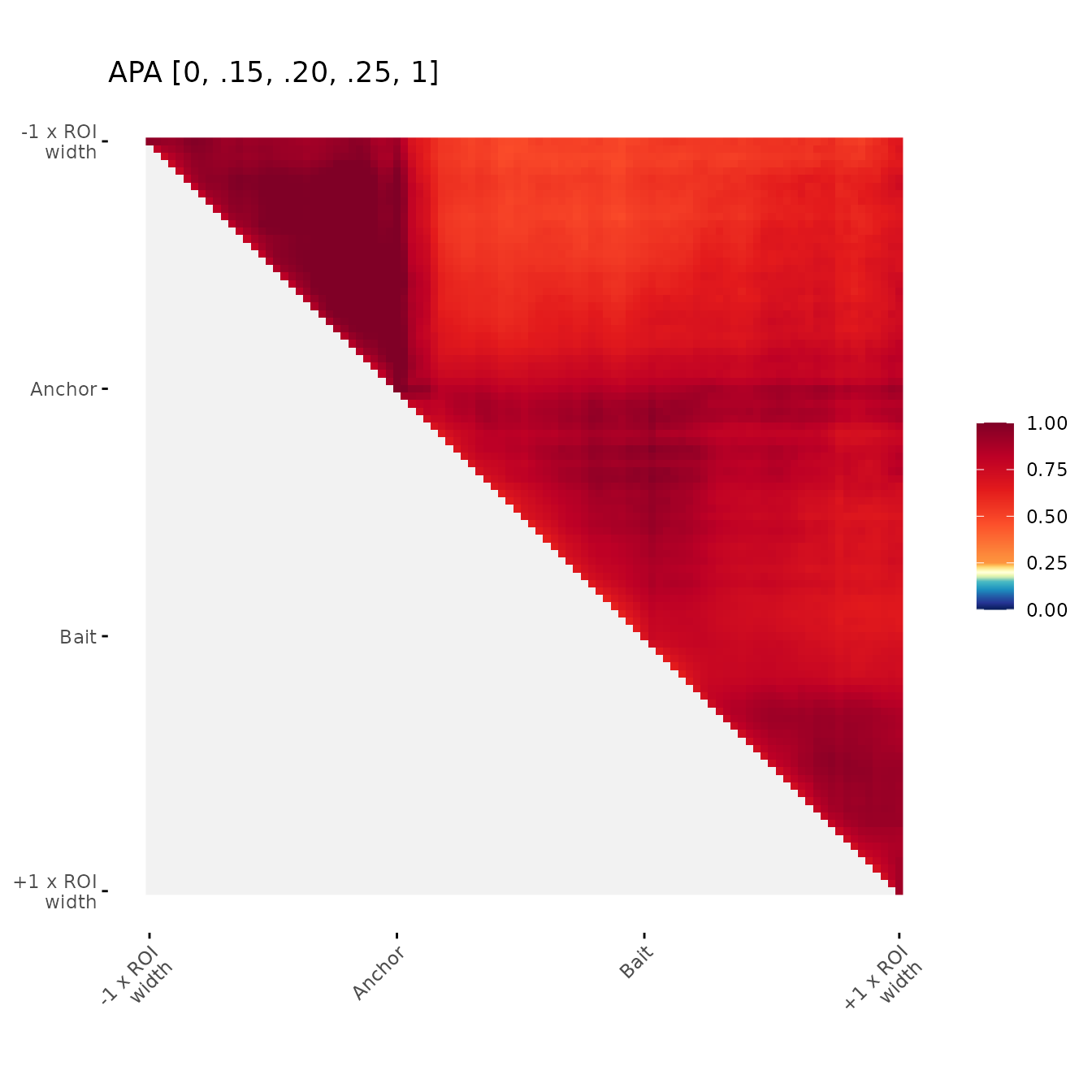
ggAPA(
        aggregatedMtx       = orientedAggreg.mtx,
        title     = "APA [0, .15, .20, .25, 1]",
        colBreaks = c(0,0.15,0.20,0.25,1)
)

ggAPA(
        aggregatedMtx       = orientedAggreg.mtx,
        title     = "APA [0, .5, .6, .8, 1]",
        colBreaks = c(0,0.4,0.5,0.7,1)
)

Change color scale bias

Examples of different color scaled bias.

ggAPA(
        aggregatedMtx    = orientedAggreg.mtx,
        title  = "APA",
        colorScale = "density"
)

ggAPA(
        aggregatedMtx     = orientedAggreg.mtx,
        title   = "APA",
        bias    = 2
)

ggAPA(
        aggregatedMtx     = orientedAggreg.mtx,
        title   = "APA",
        bias    = 0.5
)

Change color

Here is an option to change the color of heatmap and color of NA values.

ggAPA(
    aggregatedMtx     = orientedAggreg.mtx,
    title   = "APA",
    colors = viridis(6),
    na.value      = "black"
)

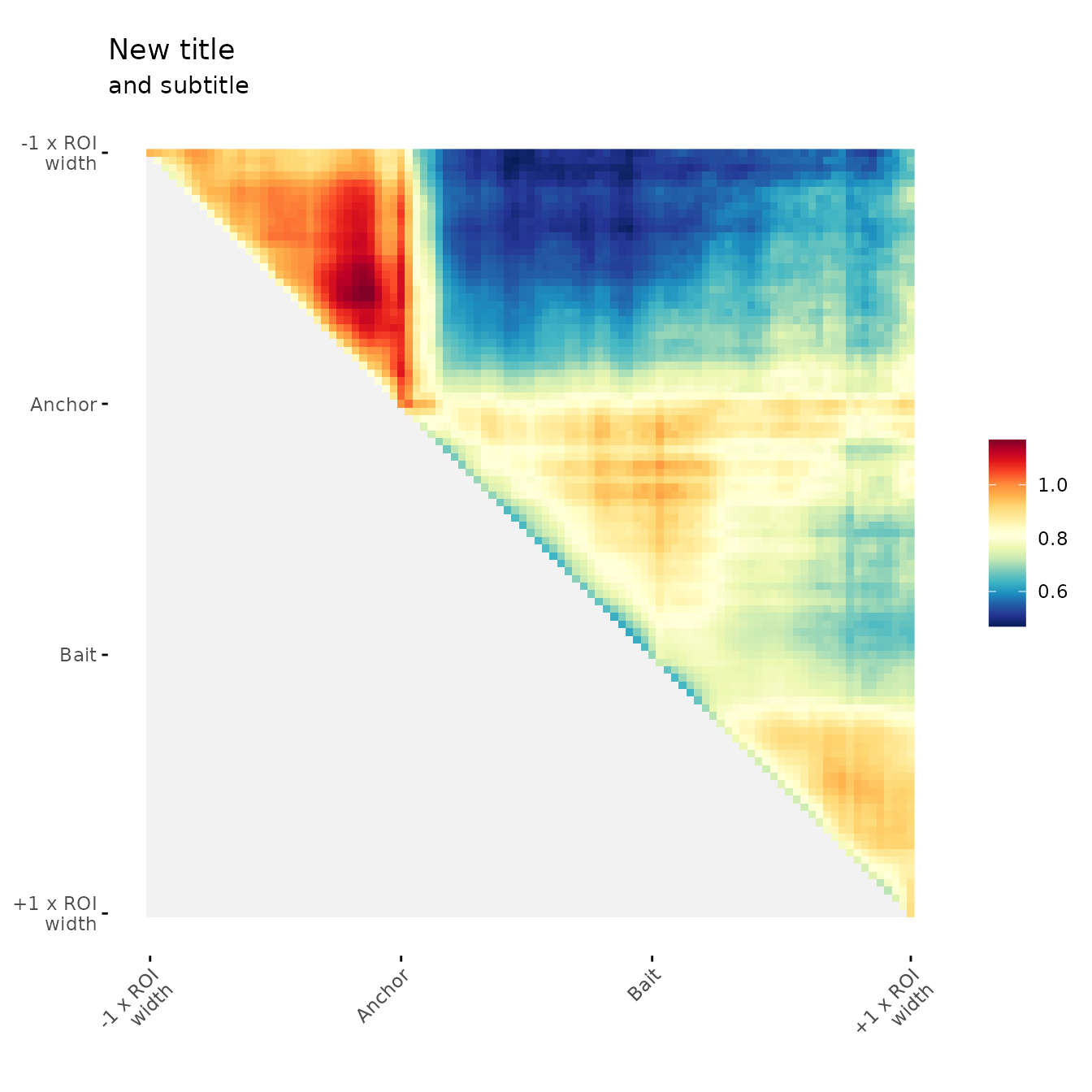
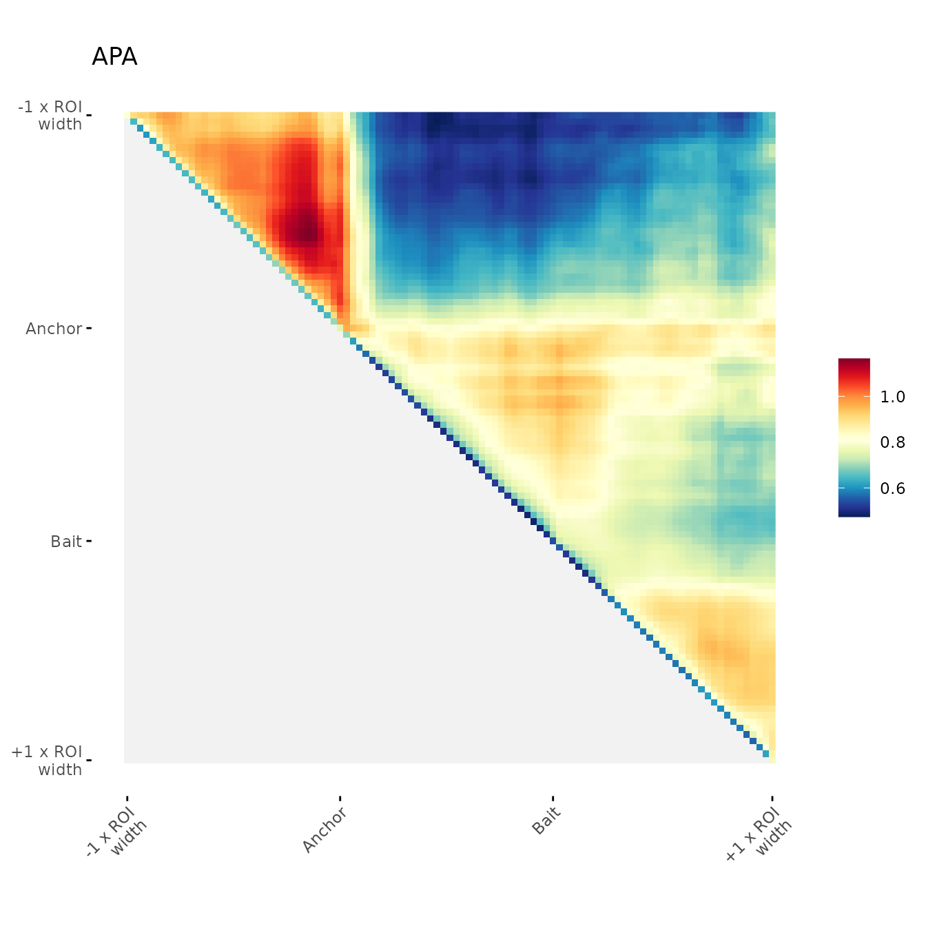
Blurred visualization

Option to apply a blurr on the heatmap to reduce noise.

ggAPA(
    aggregatedMtx           = orientedAggreg.mtx,
    title         = "APA",
    blurPass      = 1,
    stdev        = 0.5,
    loTri      = NA
)

ggplot object modifications

Since ggAPA() returns a ggplot object, it is possible to modify it following the ggplot2 grammar

ggAPA(
        aggregatedMtx     = orientedAggreg.mtx,
        title   = "APA",
) + 
ggplot2::labs(
        title    = "New title",
        subtitle = "and subtitle"
)

Session Info

sessionInfo()
#> R version 4.4.1 (2024-06-14)
#> Platform: x86_64-pc-linux-gnu
#> Running under: Ubuntu 22.04.4 LTS
#> 
#> Matrix products: default
#> BLAS:   /usr/lib/x86_64-linux-gnu/openblas-pthread/libblas.so.3 
#> LAPACK: /usr/lib/x86_64-linux-gnu/openblas-pthread/libopenblasp-r0.3.20.so;  LAPACK version 3.10.0
#> 
#> locale:
#>  [1] LC_CTYPE=C.UTF-8       LC_NUMERIC=C           LC_TIME=C.UTF-8       
#>  [4] LC_COLLATE=C.UTF-8     LC_MONETARY=C.UTF-8    LC_MESSAGES=C.UTF-8   
#>  [7] LC_PAPER=C.UTF-8       LC_NAME=C              LC_ADDRESS=C          
#> [10] LC_TELEPHONE=C         LC_MEASUREMENT=C.UTF-8 LC_IDENTIFICATION=C   
#> 
#> time zone: UTC
#> tzcode source: system (glibc)
#> 
#> attached base packages:
#> [1] stats     graphics  grDevices utils     datasets  methods   base     
#> 
#> other attached packages:
#> [1] HicAggR_1.1.3
#> 
#> loaded via a namespace (and not attached):
#>   [1] tidyselect_1.2.1            viridisLite_0.4.2          
#>   [3] farver_2.1.2                dplyr_1.1.4                
#>   [5] blob_1.2.4                  filelock_1.0.3             
#>   [7] fastmap_1.2.0               reshape_0.8.9              
#>   [9] BiocFileCache_2.12.0        digest_0.6.36              
#>  [11] lifecycle_1.0.4             RSQLite_2.3.7              
#>  [13] magrittr_2.0.3              compiler_4.4.1             
#>  [15] rlang_1.1.4                 sass_0.4.9                 
#>  [17] tools_4.4.1                 utf8_1.2.4                 
#>  [19] yaml_2.3.9                  data.table_1.15.4          
#>  [21] knitr_1.47                  labeling_0.4.3             
#>  [23] S4Arrays_1.4.1              bit_4.0.5                  
#>  [25] curl_5.2.1                  DelayedArray_0.30.1        
#>  [27] xml2_1.3.6                  plyr_1.8.9                 
#>  [29] abind_1.4-5                 BiocParallel_1.38.0        
#>  [31] withr_3.0.0                 purrr_1.0.2                
#>  [33] BiocGenerics_0.50.0         desc_1.4.3                 
#>  [35] grid_4.4.1                  stats4_4.4.1               
#>  [37] fansi_1.0.6                 colorspace_2.1-0           
#>  [39] Rhdf5lib_1.26.0             ggplot2_3.5.1              
#>  [41] scales_1.3.0                SummarizedExperiment_1.34.0
#>  [43] cli_3.6.3                   rmarkdown_2.27             
#>  [45] crayon_1.5.3                ragg_1.3.2                 
#>  [47] generics_0.1.3              rstudioapi_0.16.0          
#>  [49] httr_1.4.7                  DBI_1.2.3                  
#>  [51] cachem_1.1.0                rhdf5_2.48.0               
#>  [53] stringr_1.5.1               zlibbioc_1.50.0            
#>  [55] parallel_4.4.1              XVector_0.44.0             
#>  [57] matrixStats_1.3.0           vctrs_0.6.5                
#>  [59] Matrix_1.7-0                jsonlite_1.8.8             
#>  [61] IRanges_2.38.1              S4Vectors_0.42.1           
#>  [63] bit64_4.0.5                 systemfonts_1.1.0          
#>  [65] tidyr_1.3.1                 strawr_0.0.91              
#>  [67] jquerylib_0.1.4             glue_1.7.0                 
#>  [69] pkgdown_2.1.0               codetools_0.2-20           
#>  [71] stringi_1.8.4               gtable_0.3.5               
#>  [73] GenomeInfoDb_1.40.1         GenomicRanges_1.56.1       
#>  [75] UCSC.utils_1.0.0            munsell_0.5.1              
#>  [77] tibble_3.2.1                pillar_1.9.0               
#>  [79] htmltools_0.5.8.1           rhdf5filters_1.16.0        
#>  [81] GenomeInfoDbData_1.2.12     R6_2.5.1                   
#>  [83] dbplyr_2.5.0                textshaping_0.4.0          
#>  [85] kableExtra_1.4.0            evaluate_0.24.0            
#>  [87] lattice_0.22-6              Biobase_2.64.0             
#>  [89] highr_0.11                  backports_1.5.0            
#>  [91] memoise_2.0.1               bslib_0.7.0                
#>  [93] Rcpp_1.0.12                 InteractionSet_1.32.0      
#>  [95] svglite_2.1.3               gridExtra_2.3              
#>  [97] SparseArray_1.4.8           checkmate_2.3.1            
#>  [99] xfun_0.45                   fs_1.6.4                   
#> [101] MatrixGenerics_1.16.0       pkgconfig_2.0.3

HicAggR - In depth tutorial

Nicolas Chanard, David Depierre, Robel A. Tesfaye, Stéphane Schaak & Olivier Cuvier

2024-07-07

Introduction

Typical workflow:

Quickstart and tutorials:

Aim:

Requirements

Installation

Load library

Test dataset

Description

1. Genomic 3D structure

Temp directory preparation

Control condition (.hic File)

Heat shock condition (.mcool File)

2 Genomic location and annotation data

ChIPseq peaks of Beaf-32 protein

TSS annontation

TADs annotation

Additional genome informations

Import HiC

Import

Balancing

Tips

Observed/Expected Correction

Tips

HiC data format: ContactMatrix list structure

Indexing

Example 1: Anchors from Beaf32 ChIP-seq peaks (bed file)

Example 2: Baits from TSS (transcription start sites from UCSC)

Filter indexed features:

Tips

Search Pairs

Pairing

Tips

Extractions

Case 1: Long-range interactions between two distal anchors.

Interactions defined with GInteraction or Pairs of GRanges.

Interactions defined with GRanges.

Case 2: Interactions around genomic regions or domains.

Regions defined with GInteraction object or Pairs of GRanges

Regions defined with GRanges

Case 3: Interactions along the chromosome axis.

Example to analyse interactions in the context of TADs:

Ponctual interactions defined with GRanges

Ponctual interactions defined with GInteractions

Tips

Filtrations

Target list definition:

Example of target list:

Selection Function definition:

Example of selectionFunction according to the example target

Filtration with selection

Example of GInteraction object filtration

Example of Matrices list filtration

Specific case 1: Only one target (and therefore no selection needed)

GInteraction filtration

Matrices list filtration

Specific case 2: Sampling

GInteraction sampling

Matrices list sampling

Specific case 3: Filtration without selectionFunction

GInteraction filtration

Matrices list filtration

Tips

Selection function tips and examples:

Orientation

Information about the orientation

Orientation on matrices list

Orientation of one matrix only.

Prepare matrices list

Quantifications

Basic quantifications

Custom functions

Particular cases:

Values naming

One value extraction

Area extraction

Tips